Linear Regression Models: Diamonds Dataset.

15 minute read

1. Introduction

What is Linear Regression?

Linear regression is one of the most widely known modeling techniques in machine learning. It is usually among the first few topics people pick while learning predictive modeling. It is a method of predicting continuous values, after investigating a linear relationship between independent variables X and a dependent or response variable Y. In this type of regression, the dependent variables are continuous values while the independent variables can be either continuous, discrete or even categorical. The nature of the regression or relationship line is linear in shape, hence the name.

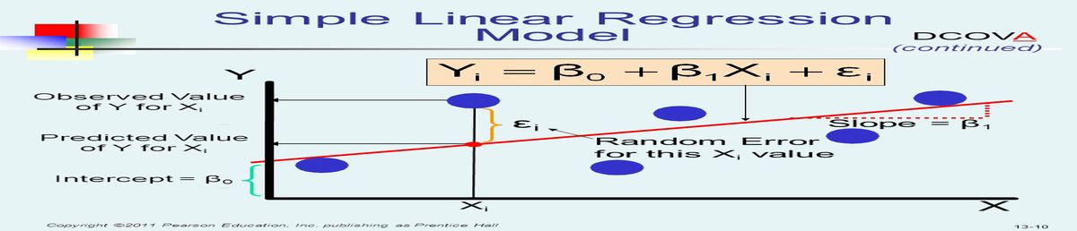
Mathematically, linear regression model is expressed as:
where y_i is an instance of y, α -the intercept of the line, indicating the value of Y when X is equal to zero, β -its slope, ε_i -its instance error and X-independent variable. α and β are generally referred to as the coefficients.

Linear Regression makes predictions by using this formula to fit a straight line to the data points in such a way that the differences between the distances of the data points from the line is minimised. Let me explain what this means literarily. Say we make a plot between carats and price from the diamonds dataset. We may get a graph as shown below.

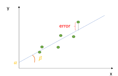
The linear line, known as best fit line, tries to draw a line in such a way that it passes through all the data points. In this case, it cannot do so without the lines becoming curvy or non-linear (This would be a non-linear regression which is out of scope of this study). Linear Regression, however, uses α and β to find the best straight line that is as closest to the points as possible. (You may have noticed that these coefficients of the line plays the most vital role in the position of the line). The difference between the best fit line and a data point is known as the error or residual or cost function. The line created above is therefore the best line it could get with the least amount of error - hence the name “best fit line”. This right here is what linear regression is all about- minimising the total amount of error between data points and its best fit line. If at this point you are asking; (a.)how can one minimise errors? (b.) How then, do we find the best values of alpha and beta in such a way that the error is minimised in order to achieve the best fit line? Then come along with me.

In this tutorial, we will use the diamonds dataset to analyse this question for predicting the price of diamonds based on a number of predictors. The main objective of this project is to review three major methods used for finding best fit line for a linear regression model in the most simplest of ways, such that a new data science enthusiast such as yourself can understand easily. The three methods we would be discussing are: Ordinary Least Squares, Gradient Descent and Regularization. But first, we have to import, clean the data and prepare it for modelling before getting to the interesting stuff. You can find more description of the dataset with this link

2. Some Data Analysis

#import helpful libraries
import numpy as np
import pandas as pd
import matplotlib.pyplot as plt
%matplotlib inline
import seaborn as sns

#get the data to work with from a link using pandas
df = pd.read_csv("https://raw.githubusercontent.com/mwaskom/seaborn-data/master/diamonds.csv")
df.sample(5) # see a sample of what's in the dataset

	carat	cut	color	clarity	depth	table	price	x	y	z
45196	0.51	Ideal	G	VS1	59.7	57.0	1656	5.20	5.25	3.12
36513	0.40	Good	I	IF	62.3	62.0	945	4.69	4.72	2.93
47927	0.56	Ideal	E	VS2	61.9	55.0	1915	5.34	5.29	3.29
46851	0.61	Premium	E	SI1	60.1	59.0	1812	5.51	5.48	3.30
31771	0.32	Premium	F	VS2	58.8	62.0	773	4.48	4.43	2.62

df.info()
# get general information about your data. How many instances? How many columns? Are there missing values?
#What type of data are the variables?

<class 'pandas.core.frame.DataFrame'>
RangeIndex: 53940 entries, 0 to 53939
Data columns (total 10 columns):
 #   Column   Non-Null Count  Dtype  
---  ------   --------------  -----  
 0   carat    53940 non-null  float64
 1   cut      53940 non-null  object
 2   color    53940 non-null  object
 3   clarity  53940 non-null  object
 4   depth    53940 non-null  float64
 5   table    53940 non-null  float64
 6   price    53940 non-null  int64  
 7   x        53940 non-null  float64
 8   y        53940 non-null  float64
 9   z        53940 non-null  float64
dtypes: float64(6), int64(1), object(3)
memory usage: 4.1+ MB

Things to note; We have approximately 54,000 instances of diamonds, no missing values and there are three object values we need to change to numeric. We change to numeric because most machine learning algorithms or models are mathematical. As such, inputs must be numerical for calculations to occur.

df.describe()

	carat	depth	table	price	x	y	z
count	53940.000000	53940.000000	53940.000000	53940.000000	53940.000000	53940.000000	53940.000000
mean	0.797940	61.749405	57.457184	3932.799722	5.731157	5.734526	3.538734
std	0.474011	1.432621	2.234491	3989.439738	1.121761	1.142135	0.705699
min	0.200000	43.000000	43.000000	326.000000	0.000000	0.000000	0.000000
25%	0.400000	61.000000	56.000000	950.000000	4.710000	4.720000	2.910000
50%	0.700000	61.800000	57.000000	2401.000000	5.700000	5.710000	3.530000
75%	1.040000	62.500000	59.000000	5324.250000	6.540000	6.540000	4.040000
max	5.010000	79.000000	95.000000	18823.000000	10.740000	58.900000	31.800000

.describe method provides some measures of variability (spread) only from the numerical variables or features. We can note that;

Max number of carat in this dataset is 5 (ughh… where are the 33 carats of Elizabeth Taylor’s??? or the 18 carats of Beyonce? can you feel my disappointment? Urrggghhh….. Anyway, at the end of this study, you can search for some celebrities independent variables online and predict their prices. See how close to the actual price you get (this is EXCERSISE ONE.)).
A large majority of the price of diamonds, (at 75th percentile), are sold at approximately 5,000USD or less.
The average depth of diamond in this dataset is 62 with its values very close to the mean.
this is not the case for price that is relatively far spread out from the mean.
Notice the min values for X, Y, Z? That tells me there are missing or unknown values present. Length, width and breadth cannot be zero… or can it? These are just some of the issues a data scientist must decide on daily basis.

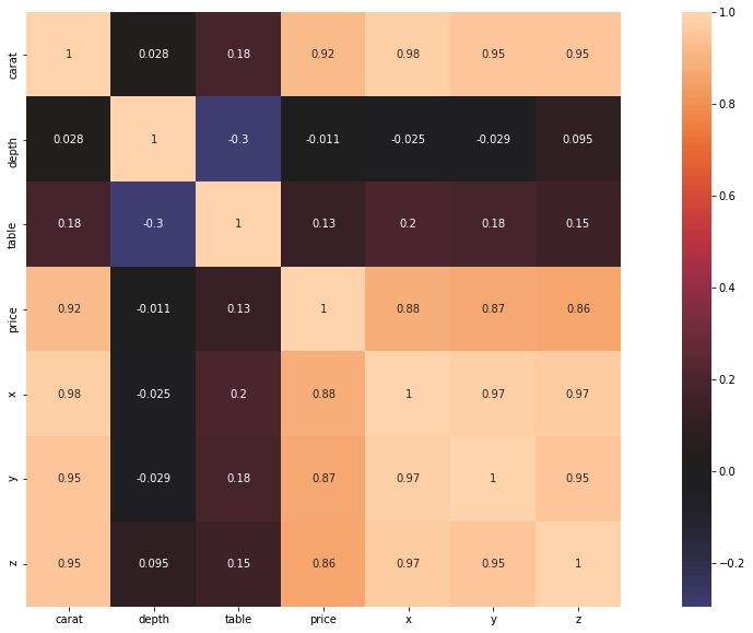
# .corr method from seaborn displays a correlation map between variables. It helps to visualise relationships between independent
# variables. In other words, it finds collinearity between variables. As a data scientist, you must decide what your threshold for
# strong collinearity is.
correlation = df.corr()

fig, ax = plt.subplots(figsize=(20,10))
sns.heatmap(correlation, center=0,  square=True,
                annot=True)
plt.show()

g = sns.pairplot(df)

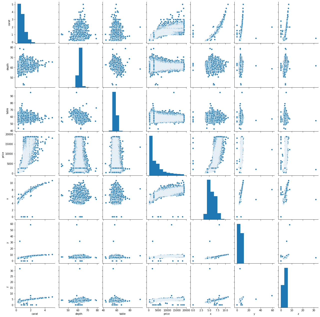
If you take a look at price, the bar chart is skewed to the right, signifying that most diamonds are bought at approximately 1500USD.
Number of Carats is the most important variable when predicting the price of diamonds while depth as well as table have little or no correlation with price.
Carat weight distribution is also right skewed portraying that majority of diamonds in the sample is on average low carat weight - 2.
Of all the dimensions of the diamond, X (length) shows the most important variable to price.

sns.relplot(x="carat", y="price", hue="color", size="cut",
            sizes=(40, 400), alpha=.5, palette="dark",
            height=6, data=df)
plt.show()

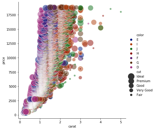
Wow! Looks like a tornado brewing. Anyway, can you see those two J colored diamonds at the top right? Good! They have the highest number of carats in the dataset, hence some of the highly priced diamonds. However, you can see that they are fairly cut. What does that tell you? That the type of cut does not really matter in terms of price? Well… not necessarily because most of the expensive ones have ideal, premium and good cuts! It would however, seem like buyers do not care so much about color.

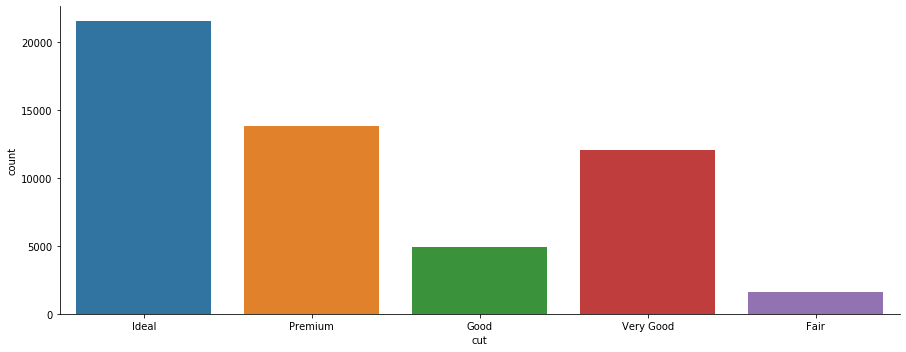
Numerical features should not have all the fun, we can also get some insights about categorical features as well.

#Seaborn's .catplot attributes shows a categorical plot. setting kind=count counts the number of unique values in a column.
sns.catplot(x='cut', data=df , kind='count',aspect=2.5 )
plt.show()

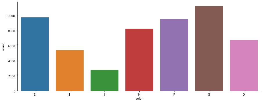
sns.catplot(x='color', kind='count', data=df, aspect=2.5 )
plt.show()

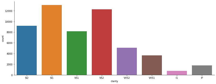
sns.catplot(x='clarity', data=df , kind='count',aspect=2.5 )
plt.show()

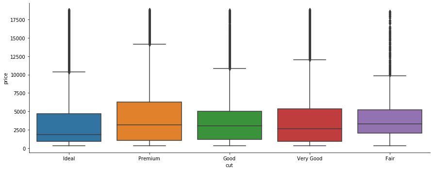
sns.catplot(x='cut', y='price', data=df, kind='box' ,aspect=2.5 )
plt.show()

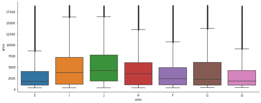
sns.catplot(x='color', y='price' , data=df , kind='box', aspect=2.5)
plt.show()

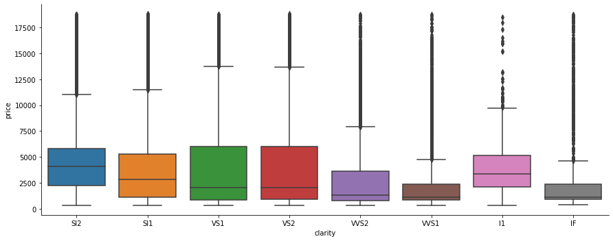
sns.catplot(x='clarity', y='price', data=df, kind='box' ,aspect=2.5 )
plt.show()

3. Data Cleaning and Preparation

df.shape #shape displays numbers of instances (horizontal), number of features/variables (vertical)

(53940, 10)

Data cleaning and preparation steps:

Find and Replace outliers.
Separate price from the other variables because it is our target.
Create train data by dropping unwanted variables. We already have price as y, we can drop Y and Z because of high collinearity with y. (Why did we keep X?).
Split dataset into train and test sets. This is done in order for the model to learn with the train set and then we check how much it has learnt with test set
Create pipeline. Read this blog post on pipelines.
- create numeric pipeline and impute missing values with iterative imputer and standardise values to remove skewness.
- create categorical variables to convert cut, color and clarity to numeric values
- add both numerical and categorical pipelines together with column transformer.

1. Find and Replace outliers.

 #first find where either of the dimensions are 0.
df.loc[(df['x']==0) | (df['y']==0) | (df['z']==0)]

	carat	cut	color	clarity	depth	table	price	x	y
2207	1.00	Premium	G	SI2	59.1	59.0	3142	6.55	6.48
2314	1.01	Premium	H	I1	58.1	59.0	3167	6.66	6.60
4791	1.10	Premium	G	SI2	63.0	59.0	3696	6.50	6.47
5471	1.01	Premium	F	SI2	59.2	58.0	3837	6.50	6.47
10167	1.50	Good	G	I1	64.0	61.0	4731	7.15	7.04
11182	1.07	Ideal	F	SI2	61.6	56.0	4954	0.00	6.62
11963	1.00	Very Good	H	VS2	63.3	53.0	5139	0.00	0.00
13601	1.15	Ideal	G	VS2	59.2	56.0	5564	6.88	6.83
15951	1.14	Fair	G	VS1	57.5	67.0	6381	0.00	0.00
24394	2.18	Premium	H	SI2	59.4	61.0	12631	8.49	8.45
24520	1.56	Ideal	G	VS2	62.2	54.0	12800	0.00	0.00
26123	2.25	Premium	I	SI1	61.3	58.0	15397	8.52	8.42
26243	1.20	Premium	D	VVS1	62.1	59.0	15686	0.00	0.00
27112	2.20	Premium	H	SI1	61.2	59.0	17265	8.42	8.37
27429	2.25	Premium	H	SI2	62.8	59.0	18034	0.00	0.00
27503	2.02	Premium	H	VS2	62.7	53.0	18207	8.02	7.95
27739	2.80	Good	G	SI2	63.8	58.0	18788	8.90	8.85
49556	0.71	Good	F	SI2	64.1	60.0	2130	0.00	0.00
49557	0.71	Good	F	SI2	64.1	60.0	2130	0.00	0.00
51506	1.12	Premium	G	I1	60.4	59.0	2383	6.71	6.67

df.loc[(df['x']==0) & (df['y']==0) & (df['z']==0)] #finds where all dimensions are zero

	carat	cut	color	clarity	depth	table	price
11963	1.00	Very Good	H	VS2	63.3	53.0	5139
15951	1.14	Fair	G	VS1	57.5	67.0	6381
24520	1.56	Ideal	G	VS2	62.2	54.0	12800
26243	1.20	Premium	D	VVS1	62.1	59.0	15686
27429	2.25	Premium	H	SI2	62.8	59.0	18034
49556	0.71	Good	F	SI2	64.1	60.0	2130
49557	0.71	Good	F	SI2	64.1	60.0	2130

#I am making a decision to drop only instances where all dimensions have 0
missing = df.loc[(df['x']==0) & (df['y']==0) & (df['z']==0)].index
df.drop(missing, inplace=True)

df.shape

(53933, 10)

print(len(df[(df['x']==0) | (df['y']==0) | (df['z']==0)])) #we can fill these with the mean

# I am replacing the 13 instances with NaN, just so an imputer finds it and treats it as missing values.
miss = df[(df['x']==0) | (df['y']==0) | (df['z']==0)]
miss.replace(0, np.NaN)

	carat	cut	color	clarity	depth	table	price	x	y	z
2207	1.00	Premium	G	SI2	59.1	59.0	3142	6.55	6.48	NaN
2314	1.01	Premium	H	I1	58.1	59.0	3167	6.66	6.60	NaN
4791	1.10	Premium	G	SI2	63.0	59.0	3696	6.50	6.47	NaN
5471	1.01	Premium	F	SI2	59.2	58.0	3837	6.50	6.47	NaN
10167	1.50	Good	G	I1	64.0	61.0	4731	7.15	7.04	NaN
11182	1.07	Ideal	F	SI2	61.6	56.0	4954	NaN	6.62	NaN
13601	1.15	Ideal	G	VS2	59.2	56.0	5564	6.88	6.83	NaN
24394	2.18	Premium	H	SI2	59.4	61.0	12631	8.49	8.45	NaN
26123	2.25	Premium	I	SI1	61.3	58.0	15397	8.52	8.42	NaN
27112	2.20	Premium	H	SI1	61.2	59.0	17265	8.42	8.37	NaN
27503	2.02	Premium	H	VS2	62.7	53.0	18207	8.02	7.95	NaN
27739	2.80	Good	G	SI2	63.8	58.0	18788	8.90	8.85	NaN
51506	1.12	Premium	G	I1	60.4	59.0	2383	6.71	6.67	NaN

2. Separate price from the other variables because it is our target.

y = df['price'].copy()

3. Create train data by dropping unwanted variables. We already have price as y, we can drop Y and Z because of high collinearity with y. (Why did we keep X?)

X = df.drop(['price', 'y', 'z'], axis=1).copy()

4. Split dataset into train and test sets. This is done in order for the model to learn with the train set and then we check how much it has learnt with test set.

from sklearn.model_selection import train_test_split

X_train, X_test, y_train, y_test = train_test_split(X, y, test_size=0.2, random_state=42)

X_train.shape

(43146, 7)

5. Create Numeric Pipeline

from sklearn.pipeline import Pipeline
from sklearn.impute import SimpleImputer
from sklearn.preprocessing import StandardScaler

train_num = X_train.select_dtypes(include=[np.number])

num_pipeline = Pipeline([
    ('imputer', SimpleImputer()),
    ('scaler', StandardScaler())
])

train_num_trx = num_pipeline.fit_transform(train_num)
train_num_trx

array([[-0.60757772, -0.31260644, -0.65357979, -0.53770462],
       [-0.83913454, -0.24256367, -1.55001822, -0.86754309],
       [ 0.46600393, -0.31260644,  2.03573552,  0.64793095],
       ...,
       [-0.96543826,  0.10765023, -0.65357979, -1.12606513],
       [ 0.21339648,  0.73803524,  0.69107786,  0.35375069],
       [ 1.03437068, -0.94299145,  0.24285865,  1.23629145]])

import category_encoders as ce

train_cat = X_train.select_dtypes(exclude=[np.number])

cat_pipeline = Pipeline([
    ('encoder', ce.OrdinalEncoder()),
    ('scaler', StandardScaler())
])
train_cat_trx = cat_pipeline.fit_transform(train_cat)
train_cat_trx.shape

(43146, 3)

from sklearn.compose import ColumnTransformer as colt

num_feats = list(train_num)
cat_feats = list(train_cat)

all_pipeline = colt([
    ('num', num_pipeline, num_feats),
    ('cat', cat_pipeline, cat_feats)
])

X_train = all_pipeline.fit_transform(X_train)
X_test = all_pipeline.transform(X_test)

X_train

array([[-0.60757772, -0.31260644, -0.65357979, ..., -1.00194956,
        -1.32387581, -2.09637234],
       [-0.83913454, -0.24256367, -1.55001822, ..., -0.11346477,
        -0.79002459, -1.4970278 ],
       [ 0.46600393, -0.31260644,  2.03573552, ...,  0.77502001,
        -0.25617336, -0.89768326],
       ...,
       [-0.96543826,  0.10765023, -0.65357979, ..., -1.00194956,
        -1.32387581, -2.09637234],
       [ 0.21339648,  0.73803524,  0.69107786, ...,  0.77502001,
         1.87923154, -0.29833873],
       [ 1.03437068, -0.94299145,  0.24285865, ...,  0.77502001,
         0.81152909,  0.90035035]])

4. Model Training

We have successfully cleaned the data, it is now ready for modeling. Going back to linear regression, I was asking how do we minimise errors or residuals to acquire the best fit line. We will now discuss some of the methods here.

4a. Ordinary Least Squares.

Remember that our goal in a multiple regression task is to minimise error term, otherwise known as optimisation. Ordinary least squares -OLS is an optimisation technique that aims to do just that. It does this by calculating the vertical distance from each data point to the fit line, squares it and sums all the squared errors together. Simple as that. In fact, Sklearn linear regression model is based on OLS. There are several measures of errors, however, we will use RMSE (Root Mean Squared Error) and R² in this project.

from sklearn.linear_model import LinearRegression
from sklearn.metrics import mean_squared_error, r2_score

linear = LinearRegression()
linear.fit(X_train, y_train)
ols_predict = linear.predict(X_test)
ols_predict

array([1037.95228275, 1141.69534609, 3535.86399969, ..., 1863.80008991,
        123.65937173, 5705.56170595])

#let us compare our real values and predicted values
print("Top 3 Labels:", list(y_test.head(3)))
print("Last 3 Labels:", list(y_test.tail(3)))

Top 3 Labels: [855, 1052, 5338]
Last 3 Labels: [1716, 457, 5006]

# mean squared error measure the average of the squares of the residual.
ols_mse = mean_squared_error(ols_predict, y_test)
ols_rmse = np.sqrt(ols_mse) #RMSE finds the square root of mse. Get it?
ols_rmse

1390.0637481799122

# R^2 also known as the coefficient of determination. It indicates how good a model/line fits the dataset.
r2_score(ols_predict, y_test)

0.8575919735124009

# this displays the coefficients of the best fit line.
linear.intercept_, linear.coef_

(3942.168775784546,
 array([ 5333.67311195,  -209.2210241 ,   -94.67012415, -1518.12967335,
         -227.21212879,  -390.0369966 ,    94.3708202 ]))

#Let us view actual and predicted values in pandas dataframe
y_test = np.array(list(y_test))

output = pd.DataFrame({'Actual':y_test.flatten(), 'Predicted':ols_predict.flatten()})
output

	Actual	Predicted
0	855	1037.952283
1	1052	1141.695346
2	5338	3535.864000
3	3465	3106.567874
4	7338	6639.779767
...	...	...
10782	12963	13359.708138
10783	2167	3019.432490
10784	1716	1863.800090
10785	457	123.659372
10786	5006	5705.561706

10787 rows × 2 columns

4b. Gradient Descent

This part aims to answer our second question. How can we optimise alpha and beta to get the least possible amount of error? One method capable of finding optimal α and β is the gradient descent algorithm. The idea is to iteratively adjust the coefficients (or weights, or parameters of the line) with the aim of minimising the cost function. It starts by initialising the weights with random values, then calculates the cost function, say with MSE. (Note how this is different from OLS where the model only find the closest vertical distance to the data points). Next, the weights are moved again ever so slightly from its initial random position towards a direction that minimises the error where the cost function is calculated again. The difference between the initial error of step 1 and this step is known as the gradient. This is done over and over till the gradient is zero or its minimum, otherwise known as global minimum. (EXERCISE 2:WHAT DO YOU THINK LOCAL MINIMUM MEANS?). If we drew a graph of movements in cost function and weights (α, β = θ), it would look like this.

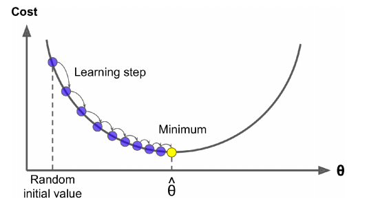I said before that we take steps ever so slightly to move the weights. How does the model determine the size of the steps then? First of all, size of steps taken is known as Learning Rate. Secondly, you determine the size of the learning rate. Thirdly, you should note that if the learning rate is too small, then the algorithm will go through many iterations to reach convergence (global minimum) which is computationally expensive. Alternatively, if the learning rate is too large, you might miss the convergence point and find your local minimum at the other side climbing up. Fourthly, when learning rate is too small, your train model will overfit(meaning it has so conformed to the patterns of the train data that it performs badly with unseen, test data). If too large, it will underfit (meaning it has not learned properly the patterns of the train data). The idea when assigning a learning rate is to find that sweet spot where it learns without overfitting.
There are two main types of gradient descent. Batch gradient descent and stochastic gradient descent. In batch GD, the path to finding a global minimum goes through very instance. Suppose you have 5million instances… Now, stochastic on the other hand locates the cost function randomly. This disadvantage here is that the model might miss its global minimum and settle for a local one. Sklearn performs a stochastic gradient descent and its learning rate is denoted as eta0.

To learn more on the mathematical derivation of gradient descent visit Anrew Ng tutorials on Coursera

from sklearn.linear_model import SGDRegressor
#This SGD runs for maximum 1,000 (indicates the number of steps it would the model to run through the train data).
#or until the loss drops by less than 0.001 during one epoch. Starting learning rate=0.05. Penalty=None:no regularisation term. More
#on this later.

sgd = SGDRegressor(max_iter=1000, tol=1e-3, penalty=None, eta0=0.05)
sgd.fit(X_train, y_train)
sgd_predict = sgd.predict(X_test)
sgd_predict

array([ 952.37745805, 1263.51124823, 3743.30446945, ..., 1931.47043363,
        171.06963592, 5941.55177469])

sgd_mse = mean_squared_error(sgd_predict, y_test)
sgd_rmse = np.sqrt(sgd_mse)
sgd_rmse

1396.8198232786256

r2_score(sgd_predict, y_test)

0.858447822595294

sgd.intercept_, sgd.coef_

(array([3944.17190108]),
 array([ 5393.05008419,  -230.92163304,  -178.24020846, -1528.70481852,
         -287.60222477,  -421.98785591,    83.26125507]))

y_test = np.array(list(y_test))

output = pd.DataFrame({'Actual':y_test.flatten(), 'Predicted':sgd_predict.flatten()})
output

	Actual	Predicted
0	855	952.377458
1	1052	1263.511248
2	5338	3743.304469
3	3465	3147.054438
4	7338	6676.896450
...	...	...
10782	12963	13270.229143
10783	2167	2900.111985
10784	1716	1931.470434
10785	457	171.069636
10786	5006	5941.551775

10787 rows × 2 columns

4c. Regularisation of Linear Regression.

A requirement for machine learning algorithm is to split a dataset into train and test sets as we had done earlier. We trained our model with the train set and made predictions with test sets that the model had not seen. Suppose we are comparing two machine learning models where one is Ordinary Least Squares-Model A and another model say model B. We found earlier that no matter how much we try to fit the line in training, it could never be curvy. In other words, it could never capture all the properties or the true values of the train dataset. This inability for OLS and other linear machine learning models is called Bias and they are usually high. Suppose our other model B during training, is super flexible and captures the true nature of relationships in the dataset. If you calculate the cost function of both models at training, model B would win because of its incredible low or zero bias. Next stage in machine learning is to predict on test sets. When you fit both models to the test sets, OLS wins. This is because the second model overfit (that is, it captured every noise, bias or error in the train data), therefore could not generalise to a new (test) set. The difference in cost acquired during train and test sets is called Variance. Our second hypothetical model has a high variance because while it suggested good results in training (low bias), it would perform poorly in generalisation. Lets review these lines for visual explanation.

Source

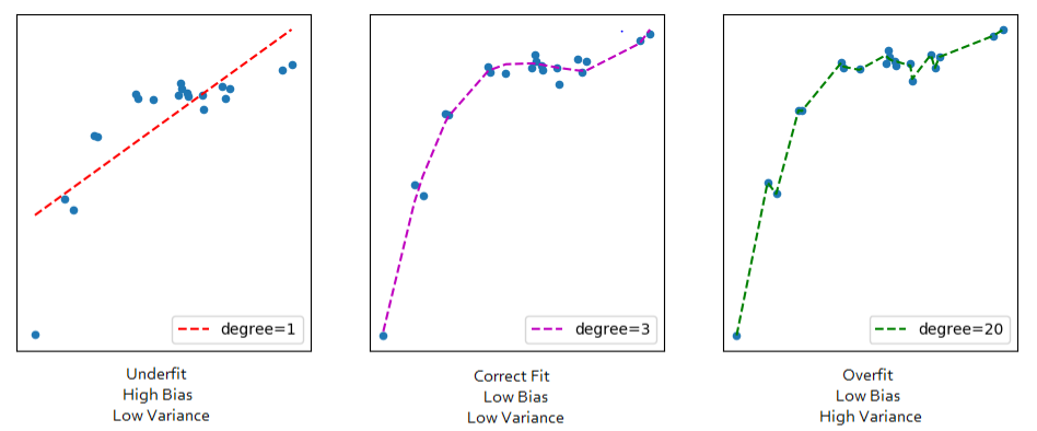
As a data scientist, you want your model to have low bias as well as low variance (correct fit). Low bias means it does not underfit, it learns well enough of the train data and low variance means it does not overfit, it does not over learn. Therefore, as the bias increases, the lower the variance gets. But we want the bias to be low as well… hmmm… How is this possible? Answer to this question is referred as the Bias-Variance Tradeoff. Some of the methods for finding a correct fit is Bagging, Boosting and Regularisation. In this section, we will treat three Regularisation methods. They are; Ridge Regression, Lasso Regression and ElasticNet. Other non-linear Regularization methods will be discussed in later posts.

4c.1. Ridge Regression

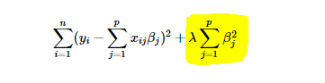
In the example above, we have assumed that the dataset presented to OLS has high bias. What about in situations where the line captures the true nature of the train dataset? (I know this is inconceivable but walk with me). In other words, the model has relatively low bias, high variance? Ridge regression also known as L2 regularisation, provides a solution. The idea of ridge regression is to find a line that does not fit to the train data so well by shrinking its parameters towards zero. Yes, it intentionally reduces fitness. This objective is to help it generalise well to unseen data. It does this by introducing a small amount of bias when fitting a line. Because of the introduced amount of bias, a significant drop in variance is also achieved. When OLS estimates the values of its parameters, it minimises error by summing the square residuals. However, in ridge regression, it does the same thing but adds λ * β², also known as ridge regression penalty.

By intuition, when λ is 0, we still have OLS. However, as λ increases, fitness reduces. How then can we decide the optimal value of λ? Different values are tried in cross-validation to determine the value that results in the least amount of variance. We should not expect it to perform better in our diamonds project because we suspect our dataset to have high bias already.
To find out if your data has high bias, predict on train set. If your cost function increases, then you have high bias.

from sklearn.linear_model import RidgeCV

ridge = RidgeCV(alphas=[1.0, 100.0, 1000.0])#obviously 1.0 is the least alpha-regularisation term for the least variance. check with just the other values. See how rmse changes.
ridge.fit(X_train, y_train)
ridge_predict = ridge.predict(X_test)
ridge_predict

array([1037.73541556, 1141.05217163, 3536.43927354, ..., 1864.14253671,
        123.00128024, 5706.39133431])

ridge_mse = mean_squared_error(ridge_predict, y_test)
ridge_rmse = np.sqrt(ridge_mse)
ridge_rmse

1390.0796687381596

r2_score(ridge_predict, y_test)

0.8575751475226532

As noted earlier, OLS model already underfits, hence there would be no need to add more bias. This is why we have the same result as the OLS model.

4c.2. Lasso Regression

Lasso Regression also known as L1 Regularisation is somewhat similar to ridge regression in that they both add penalty to least squares. However, where ridge squares β, lasso estimates the absolute value of β.

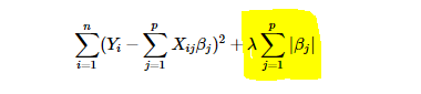
LASSO - Least Absolute Shrinkage and Selection Operator is a powerful method that perform two main tasks - regularisation and feature selection. The LASSO method puts a constraint on the sum of the absolute values of the model parameters. The sum has to be less than a fixed value (upper bound). In order to do so the method applies a shrinking (regularization) process where it penalizes the coefficients of the regression variables shrinking some of them to zero. During features selection process the variables that still have a non-zero coefficient after the shrinking process are selected to be part of the model. The goal of this process is to minimize the prediction error. In practice the tuning parameter λ, that controls the strength of the penalty, assume a great importance. Indeed when λ is sufficiently large then coefficients are forced to be exactly equal to zero, this way dimensionality can be reduced. The larger is the parameter λ the more number of coefficients are reduced to zero. On the other hand if λ = 0 we have an OLS (Ordinary Least Square) regression. lasso regression works best when your dataset contains useless variables. it helps to weed out the useless ones and keeps the important ones. since we do not have any useless variable, we can assume that our prediction would be similar to ridge regression.

from sklearn.linear_model import Lasso
lasso = Lasso()
lasso.fit(X_train, y_train)
lasso_pred = lasso.predict(X_test)
lasso_pred

array([1035.49937663, 1132.39269291, 3543.13949262, ..., 1867.37944786,
        113.75699813, 5714.87134798])

lasso_mse = mean_squared_error(lasso_pred, y_test)
lasso_rmse = np.sqrt(lasso_mse)
lasso_rmse

1390.3302835348156

r2_score(lasso_pred, y_test)

0.8573885427837196

4c.3. Elastic-Net Regression

We concluded earlier that while ridge regression works best for dataset where most of the variables in the model are useful, lasso regression works best when most are useless. However, what do you do when your dataset has thousands of variables without knowing in advance the type of dataset? Elastic-net regression to the rescue. Just like ridge and Lasso, elastic regression starts with least squares, then combines the penalties of Ridge and Lasso together. However, Lasso and Ridge penalties get their own λs. Cross validation on different combinations of λs to find the best values.

from sklearn.linear_model import ElasticNet

elastic = ElasticNet(random_state=42)
elastic.fit(X_train, y_train)
elastic_pred = elastic.predict(X_test)
elastic_pred

array([1431.38133481, 1045.02625539, 3700.72105628, ..., 2353.89127405,
        535.08437658, 5697.14712005])

elastic_mse = mean_squared_error(elastic_pred, y_test)
elastic_rmse = np.sqrt(elastic_mse)
elastic_rmse

1734.5381855308262

r2_score(elastic_pred, y_test)

0.6348536268574031

Conclusion.

We have come to the end of our Linear Regression tutorial. If you understand all the algorithms mentioned here, then you are at an intermediate level. If you can create the mathematical deductions, well, what an expert. Kudos to you all. On a serious note, we have learnt about Linear Regression and also reviewed its flaws which predominantly refers to its inherent high bias nature. The only solution for an underfitting model is to use a more complex model as is our case study. If it were overfitting, then L1 and L2 regularisation would have produced better results. Next is classification models. Link

Thank you for reading, Bye for now.

Share on

Twitter Facebook LinkedIn

Misan Daibo