Kaggle: Ames_Housing

This is a Kaggle project tutorial that predicts Ames Iowa houses.

Head to Kaggle to get a full description of this dataset.

1. Generate an idea

Firstly, it is always good practice to have knowledge of what the objective of the project is. This means analysing who/what/where/when stands to benefit from your outcome. It helps you understand as well as create a guideline for the problem on a personal scale.  
For this project, let us assume we are working for  real estate investors who would like to predict the SalePrice of houses in Ames, Iowa, given 80 factors or predictor variables. They would like to know if investing would be a good business idea. With this in mind, you can start thinking of types of information you could provide your employer that would help them gain competitive advantage. How would you deliver your findings to a non-science audience? You should develop these thought processes from the beginning.
At this point, if you have previewed the data, you can tell that this is a batch univariate regression problem. Although RMSE has been chosen as its performance measure, note that if there are lots of outliers, you could also try MAE.  

2. Load the data

#first, we load libraries
import numpy as np
import pandas as pd
import matplotlib.pyplot as plt
%matplotlib inline
import seaborn as sns
import warnings
warnings.filterwarnings(action="ignore", message="^internal gelsd")
warnings.simplefilter(action='ignore', category=FutureWarning)

#load data
train_df = pd.read_csv("train.csv")
test_df = pd.read_csv("test.csv")
sub_df = pd.read_csv("sample_submission.csv")

pd.set_option('display.max_columns', None)
train_df.sample(5)

	Id	MSSubClass	MSZoning	LotFrontage	LotArea	Street	Alley	LotShape	LandContour	Utilities	LotConfig	LandSlope	Neighborhood	Condition1	Condition2	BldgType	HouseStyle	OverallQual	OverallCond	YearBuilt	YearRemodAdd	RoofStyle	RoofMatl	Exterior1st	Exterior2nd	MasVnrType	MasVnrArea	ExterQual	ExterCond	Foundation	BsmtQual	BsmtCond	BsmtExposure	BsmtFinType1	BsmtFinSF1	BsmtFinType2	BsmtFinSF2	BsmtUnfSF	TotalBsmtSF	Heating	HeatingQC	CentralAir	Electrical	1stFlrSF	2ndFlrSF	LowQualFinSF	GrLivArea	BsmtFullBath	BsmtHalfBath	FullBath	HalfBath	BedroomAbvGr	KitchenAbvGr	KitchenQual	TotRmsAbvGrd	Functional	Fireplaces	FireplaceQu	GarageType	GarageYrBlt	GarageFinish	GarageCars	GarageArea	GarageQual	GarageCond	PavedDrive	WoodDeckSF	OpenPorchSF	EnclosedPorch	3SsnPorch	ScreenPorch	PoolArea	PoolQC	Fence	MiscFeature	MiscVal	MoSold	YrSold	SaleType	SaleCondition	SalePrice
1038	1039	160	RM	21.0	1533	Pave	NaN	Reg	Lvl	AllPub	Inside	Gtl	MeadowV	Norm	Norm	Twnhs	2Story	4	6	1970	2008	Gable	CompShg	CemntBd	CmentBd	None	0.0	TA	TA	CBlock	TA	TA	No	Unf	0	Unf	0	546	546	GasA	TA	Y	SBrkr	798	546	0	1344	0	0	1	1	3	1	TA	6	Typ	1	TA	NaN	NaN	NaN	0	0	NaN	NaN	Y	0	0	0	0	0	0	NaN	NaN	NaN	0	5	2009	WD	Normal	97000
828	829	60	RL	NaN	28698	Pave	NaN	IR2	Low	AllPub	CulDSac	Sev	ClearCr	Norm	Norm	1Fam	2Story	5	5	1967	1967	Flat	Tar&Grv	Plywood	Plywood	None	0.0	TA	TA	PConc	TA	Gd	Gd	LwQ	249	ALQ	764	0	1013	GasA	TA	Y	SBrkr	1160	966	0	2126	0	1	2	1	3	1	TA	7	Min2	0	NaN	Attchd	1967.0	Fin	2	538	TA	TA	Y	486	0	0	0	225	0	NaN	NaN	NaN	0	6	2009	WD	Abnorml	185000
174	175	20	RL	47.0	12416	Pave	NaN	IR1	Lvl	AllPub	Inside	Gtl	Timber	Norm	Norm	1Fam	1Story	6	5	1986	1986	Gable	CompShg	VinylSd	Plywood	Stone	132.0	TA	TA	CBlock	Gd	Fa	No	ALQ	1398	LwQ	208	0	1606	GasA	TA	Y	SBrkr	1651	0	0	1651	1	0	2	0	3	1	TA	7	Min2	1	TA	Attchd	1986.0	Fin	2	616	TA	TA	Y	192	0	0	0	0	0	NaN	NaN	NaN	0	11	2008	WD	Normal	184000
534	535	60	RL	74.0	9056	Pave	NaN	IR1	Lvl	AllPub	Inside	Gtl	Gilbert	Norm	Norm	1Fam	2Story	8	5	2004	2004	Gable	CompShg	VinylSd	VinylSd	None	0.0	Gd	TA	PConc	Ex	Gd	Av	Unf	0	Unf	0	707	707	GasA	Ex	Y	SBrkr	707	707	0	1414	0	0	2	1	3	1	Gd	6	Typ	1	Gd	Attchd	2004.0	Fin	2	403	TA	TA	Y	100	35	0	0	0	0	NaN	NaN	NaN	0	10	2006	WD	Normal	178000
443	444	120	RL	53.0	3922	Pave	NaN	Reg	Lvl	AllPub	Inside	Gtl	Blmngtn	Norm	Norm	TwnhsE	1Story	7	5	2006	2007	Gable	CompShg	WdShing	Wd Shng	BrkFace	72.0	Gd	TA	PConc	Ex	TA	Av	Unf	0	Unf	0	1258	1258	GasA	Ex	Y	SBrkr	1258	0	0	1258	0	0	2	0	2	1	Gd	6	Typ	1	Gd	Attchd	2007.0	Fin	3	648	TA	TA	Y	144	16	0	0	0	0	NaN	NaN	NaN	0	6	2007	New	Partial	172500

print(train_df.shape)
print(test_df.shape)

(1460, 81)
(1459, 80)

3. Analyze and Visualize Data

This stage provides an oppurtunity to gain some meaningful insights and get a statistical ‘feel’ of hidden elements in the data.

train_df.info()

<class 'pandas.core.frame.DataFrame'>
RangeIndex: 1460 entries, 0 to 1459
Data columns (total 81 columns):
 #   Column         Non-Null Count  Dtype  
---  ------         --------------  -----  
 0   Id             1460 non-null   int64  
 1   MSSubClass     1460 non-null   int64  
 2   MSZoning       1460 non-null   object
 3   LotFrontage    1201 non-null   float64
 4   LotArea        1460 non-null   int64  
 5   Street         1460 non-null   object
 6   Alley          91 non-null     object
 7   LotShape       1460 non-null   object
 8   LandContour    1460 non-null   object
 9   Utilities      1460 non-null   object
 10  LotConfig      1460 non-null   object
 11  LandSlope      1460 non-null   object
 12  Neighborhood   1460 non-null   object
 13  Condition1     1460 non-null   object
 14  Condition2     1460 non-null   object
 15  BldgType       1460 non-null   object
 16  HouseStyle     1460 non-null   object
 17  OverallQual    1460 non-null   int64  
 18  OverallCond    1460 non-null   int64  
 19  YearBuilt      1460 non-null   int64  
 20  YearRemodAdd   1460 non-null   int64  
 21  RoofStyle      1460 non-null   object
 22  RoofMatl       1460 non-null   object
 23  Exterior1st    1460 non-null   object
 24  Exterior2nd    1460 non-null   object
 25  MasVnrType     1452 non-null   object
 26  MasVnrArea     1452 non-null   float64
 27  ExterQual      1460 non-null   object
 28  ExterCond      1460 non-null   object
 29  Foundation     1460 non-null   object
 30  BsmtQual       1423 non-null   object
 31  BsmtCond       1423 non-null   object
 32  BsmtExposure   1422 non-null   object
 33  BsmtFinType1   1423 non-null   object
 34  BsmtFinSF1     1460 non-null   int64  
 35  BsmtFinType2   1422 non-null   object
 36  BsmtFinSF2     1460 non-null   int64  
 37  BsmtUnfSF      1460 non-null   int64  
 38  TotalBsmtSF    1460 non-null   int64  
 39  Heating        1460 non-null   object
 40  HeatingQC      1460 non-null   object
 41  CentralAir     1460 non-null   object
 42  Electrical     1459 non-null   object
 43  1stFlrSF       1460 non-null   int64  
 44  2ndFlrSF       1460 non-null   int64  
 45  LowQualFinSF   1460 non-null   int64  
 46  GrLivArea      1460 non-null   int64  
 47  BsmtFullBath   1460 non-null   int64  
 48  BsmtHalfBath   1460 non-null   int64  
 49  FullBath       1460 non-null   int64  
 50  HalfBath       1460 non-null   int64  
 51  BedroomAbvGr   1460 non-null   int64  
 52  KitchenAbvGr   1460 non-null   int64  
 53  KitchenQual    1460 non-null   object
 54  TotRmsAbvGrd   1460 non-null   int64  
 55  Functional     1460 non-null   object
 56  Fireplaces     1460 non-null   int64  
 57  FireplaceQu    770 non-null    object
 58  GarageType     1379 non-null   object
 59  GarageYrBlt    1379 non-null   float64
 60  GarageFinish   1379 non-null   object
 61  GarageCars     1460 non-null   int64  
 62  GarageArea     1460 non-null   int64  
 63  GarageQual     1379 non-null   object
 64  GarageCond     1379 non-null   object
 65  PavedDrive     1460 non-null   object
 66  WoodDeckSF     1460 non-null   int64  
 67  OpenPorchSF    1460 non-null   int64  
 68  EnclosedPorch  1460 non-null   int64  
 69  3SsnPorch      1460 non-null   int64  
 70  ScreenPorch    1460 non-null   int64  
 71  PoolArea       1460 non-null   int64  
 72  PoolQC         7 non-null      object
 73  Fence          281 non-null    object
 74  MiscFeature    54 non-null     object
 75  MiscVal        1460 non-null   int64  
 76  MoSold         1460 non-null   int64  
 77  YrSold         1460 non-null   int64  
 78  SaleType       1460 non-null   object
 79  SaleCondition  1460 non-null   object
 80  SalePrice      1460 non-null   int64  
dtypes: float64(3), int64(35), object(43)
memory usage: 924.0+ KB

The first thing you notice is, there is a significant number of object type values in the data.
Also, Alley, PoolQC, Fence and MiscFeature, have a considerable number of missing values.

train_df.describe().T #This displays a statistical summary of numerical variables.

	count	mean	std	min	25%	50%	75%	max
Id	1460.0	730.500000	421.610009	1.0	365.75	730.5	1095.25	1460.0
MSSubClass	1460.0	56.897260	42.300571	20.0	20.00	50.0	70.00	190.0
LotFrontage	1201.0	70.049958	24.284752	21.0	59.00	69.0	80.00	313.0
LotArea	1460.0	10516.828082	9981.264932	1300.0	7553.50	9478.5	11601.50	215245.0
OverallQual	1460.0	6.099315	1.382997	1.0	5.00	6.0	7.00	10.0
OverallCond	1460.0	5.575342	1.112799	1.0	5.00	5.0	6.00	9.0
YearBuilt	1460.0	1971.267808	30.202904	1872.0	1954.00	1973.0	2000.00	2010.0
YearRemodAdd	1460.0	1984.865753	20.645407	1950.0	1967.00	1994.0	2004.00	2010.0
MasVnrArea	1452.0	103.685262	181.066207	0.0	0.00	0.0	166.00	1600.0
BsmtFinSF1	1460.0	443.639726	456.098091	0.0	0.00	383.5	712.25	5644.0
BsmtFinSF2	1460.0	46.549315	161.319273	0.0	0.00	0.0	0.00	1474.0
BsmtUnfSF	1460.0	567.240411	441.866955	0.0	223.00	477.5	808.00	2336.0
TotalBsmtSF	1460.0	1057.429452	438.705324	0.0	795.75	991.5	1298.25	6110.0
1stFlrSF	1460.0	1162.626712	386.587738	334.0	882.00	1087.0	1391.25	4692.0
2ndFlrSF	1460.0	346.992466	436.528436	0.0	0.00	0.0	728.00	2065.0
LowQualFinSF	1460.0	5.844521	48.623081	0.0	0.00	0.0	0.00	572.0
GrLivArea	1460.0	1515.463699	525.480383	334.0	1129.50	1464.0	1776.75	5642.0
BsmtFullBath	1460.0	0.425342	0.518911	0.0	0.00	0.0	1.00	3.0
BsmtHalfBath	1460.0	0.057534	0.238753	0.0	0.00	0.0	0.00	2.0
FullBath	1460.0	1.565068	0.550916	0.0	1.00	2.0	2.00	3.0
HalfBath	1460.0	0.382877	0.502885	0.0	0.00	0.0	1.00	2.0
BedroomAbvGr	1460.0	2.866438	0.815778	0.0	2.00	3.0	3.00	8.0
KitchenAbvGr	1460.0	1.046575	0.220338	0.0	1.00	1.0	1.00	3.0
TotRmsAbvGrd	1460.0	6.517808	1.625393	2.0	5.00	6.0	7.00	14.0
Fireplaces	1460.0	0.613014	0.644666	0.0	0.00	1.0	1.00	3.0
GarageYrBlt	1379.0	1978.506164	24.689725	1900.0	1961.00	1980.0	2002.00	2010.0
GarageCars	1460.0	1.767123	0.747315	0.0	1.00	2.0	2.00	4.0
GarageArea	1460.0	472.980137	213.804841	0.0	334.50	480.0	576.00	1418.0
WoodDeckSF	1460.0	94.244521	125.338794	0.0	0.00	0.0	168.00	857.0
OpenPorchSF	1460.0	46.660274	66.256028	0.0	0.00	25.0	68.00	547.0
EnclosedPorch	1460.0	21.954110	61.119149	0.0	0.00	0.0	0.00	552.0
3SsnPorch	1460.0	3.409589	29.317331	0.0	0.00	0.0	0.00	508.0
ScreenPorch	1460.0	15.060959	55.757415	0.0	0.00	0.0	0.00	480.0
PoolArea	1460.0	2.758904	40.177307	0.0	0.00	0.0	0.00	738.0
MiscVal	1460.0	43.489041	496.123024	0.0	0.00	0.0	0.00	15500.0
MoSold	1460.0	6.321918	2.703626	1.0	5.00	6.0	8.00	12.0
YrSold	1460.0	2007.815753	1.328095	2006.0	2007.00	2008.0	2009.00	2010.0
SalePrice	1460.0	180921.195890	79442.502883	34900.0	129975.00	163000.0	214000.00	755000.0

Just from looking at this we can make quick simple basic inferences such as, half the number of houses were built in 1973 or earlier; the mean over all quality of houses sold is 6; there are no duplexes in 75% of houses sold; first remodelling was in 1950. For the target variable, minimum value of house sold is 34,900 dollars with maximum value of 755,000 dollars and mean of 163,000; A quarter of the houses are sold at about 130,000 or lower. Go ahead, make some conjectures of your own.

# lets see what we can find from our object type variables
train_df.describe(include = [np.object])

	MSZoning	Street	Alley	LotShape	LandContour	Utilities	LotConfig	LandSlope	Neighborhood	Condition1	Condition2	BldgType	HouseStyle	RoofStyle	RoofMatl	Exterior1st	Exterior2nd	MasVnrType	ExterQual	ExterCond	Foundation	BsmtQual	BsmtCond	BsmtExposure	BsmtFinType1	BsmtFinType2	Heating	HeatingQC	CentralAir	Electrical	KitchenQual	Functional	FireplaceQu	GarageType	GarageFinish	GarageQual	GarageCond	PavedDrive	PoolQC	Fence	MiscFeature	SaleType	SaleCondition
count	1460	1460	91	1460	1460	1460	1460	1460	1460	1460	1460	1460	1460	1460	1460	1460	1460	1452	1460	1460	1460	1423	1423	1422	1423	1422	1460	1460	1460	1459	1460	1460	770	1379	1379	1379	1379	1460	7	281	54	1460	1460
unique	5	2	2	4	4	2	5	3	25	9	8	5	8	6	8	15	16	4	4	5	6	4	4	4	6	6	6	5	2	5	4	7	5	6	3	5	5	3	3	4	4	9	6
top	RL	Pave	Grvl	Reg	Lvl	AllPub	Inside	Gtl	NAmes	Norm	Norm	1Fam	1Story	Gable	CompShg	VinylSd	VinylSd	None	TA	TA	PConc	TA	TA	No	Unf	Unf	GasA	Ex	Y	SBrkr	TA	Typ	Gd	Attchd	Unf	TA	TA	Y	Gd	MnPrv	Shed	WD	Normal
freq	1151	1454	50	925	1311	1459	1052	1382	225	1260	1445	1220	726	1141	1434	515	504	864	906	1282	647	649	1311	953	430	1256	1428	741	1365	1334	735	1360	380	870	605	1311	1326	1340	3	157	49	1267	1198

Unlike describe method for numerical values, this only shows count (total number of instances), unique (number of unique values), top (most occurring attribute) and frequency (Frequency of top values). You can deduce observations such as; 99.5% of streets are paved, as should be expected; 79% of houses sold are in low population density residential areas (RL) and that 51% of houses bought had excellent heating quality (HeatingQC)of gas forced air and so on.
Next step is to push your analysis further by visualizing sections of the dtypes to get more and better insights, especially to find trends and patterns that may indicate a relationship.

#first let us find the most correlated of attributes to our target variable since we cannot possibly plot all features.
corr = train_df.corr()
corr["SalePrice"].sort_values(ascending=False)

SalePrice        1.000000
OverallQual      0.790982
GrLivArea        0.708624
GarageCars       0.640409
GarageArea       0.623431
TotalBsmtSF      0.613581
1stFlrSF         0.605852
FullBath         0.560664
TotRmsAbvGrd     0.533723
YearBuilt        0.522897
YearRemodAdd     0.507101
GarageYrBlt      0.486362
MasVnrArea       0.477493
Fireplaces       0.466929
BsmtFinSF1       0.386420
LotFrontage      0.351799
WoodDeckSF       0.324413
2ndFlrSF         0.319334
OpenPorchSF      0.315856
HalfBath         0.284108
LotArea          0.263843
BsmtFullBath     0.227122
BsmtUnfSF        0.214479
BedroomAbvGr     0.168213
ScreenPorch      0.111447
PoolArea         0.092404
MoSold           0.046432
3SsnPorch        0.044584
BsmtFinSF2      -0.011378
BsmtHalfBath    -0.016844
MiscVal         -0.021190
Id              -0.021917
LowQualFinSF    -0.025606
YrSold          -0.028923
OverallCond     -0.077856
MSSubClass      -0.084284
EnclosedPorch   -0.128578
KitchenAbvGr    -0.135907
Name: SalePrice, dtype: float64

Well, there you have it. These are the most positively and negatively correlated attributes with respect to price of houses in Ames. The negative correlations are very close to zero; as such, ineligible. We can ignore them for now. Let us go ahead and visualize some of pos_corr to show if there are any linear relationships present.

sns.set(palette="deep", font_scale=1.0)        

select_corr = ["OverallQual", "GrLivArea", "GarageCars", "GarageArea",
               "TotalBsmtSF", "1stFlrSF","FullBath", "TotRmsAbvGrd", "YearBuilt",
               "YearRemodAdd","GarageYrBlt", "EnclosedPorch", "KitchenAbvGr", "MSSubClass", "LowQualFinSF"]

fig, ax = plt.subplots(5, 3, figsize=(20, 35))
for var, subplot in zip(select_corr, ax.flatten()):
    sns.scatterplot(x=var, y='SalePrice' , hue='MSZoning', data=train_df, ax=subplot)
    for label in subplot.get_xticklabels():
        label.set_rotation(90)

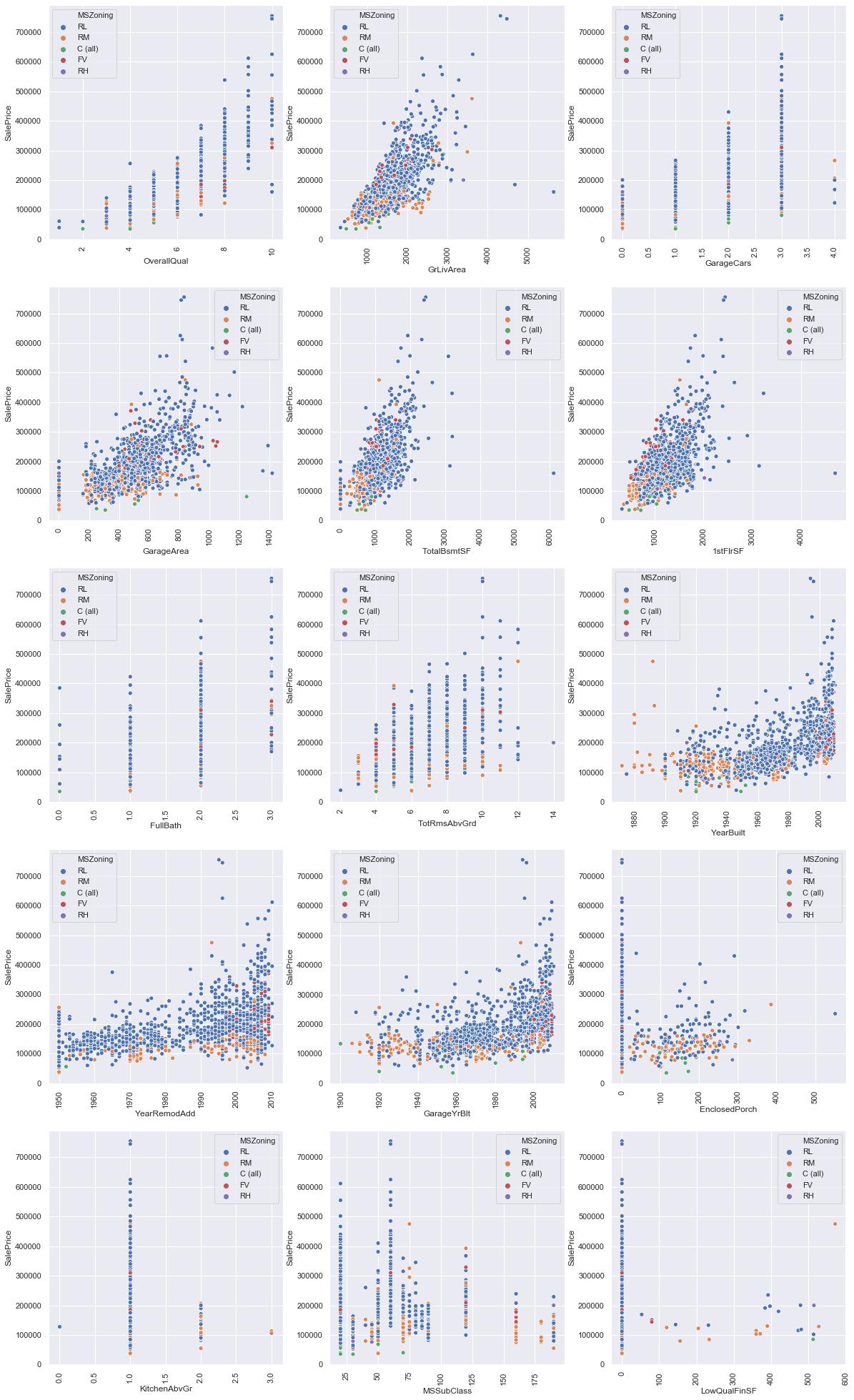
First thing you can notice is that most of the plots show positive linear relationships. There is also a large disparity in values between some independent variables and the target variable. This needs to be taken care of at a later stage. Next, as expected, we can see that when overall quality increases, the price goes up; Most of the houses are located at the RL zoning classification; Houses in commercial areas (C) are the cheapest as they seem to have lowest overall quality; Houses in low residential density areas (RL) have higher above ground living area, larger garage in size and number of cars it can contain and boasts of the most expensive houses; Houses in RM & C zoning classification have the smallest average of total basement area; Highest grade bathrooms starts at approximately $180,000; only one instance of 14 rooms in the training dataset; and so on. It is also quite evident that some of the variables are not uniformly distributed. Next we take a look at the relationship between some randomly selected categorical variables and the target variable.

sns.set(palette="deep", font_scale=1.0)        

select_var = [
  'MSZoning', 'LotShape', 'Neighborhood', 'Condition2', 'SaleCondition', 'BsmtCond', 'ExterCond',
    "MasVnrType", "Condition1", "KitchenQual", 'BldgType', 'Functional'
]
fig, ax = plt.subplots(4, 3, figsize=(20, 35))
for var, subplot in zip(select_var, ax.flatten()):
    sns.boxplot(x=var, y='SalePrice', data=train_df, ax=subplot)
    for label in subplot.get_xticklabels():
        label.set_rotation(90)

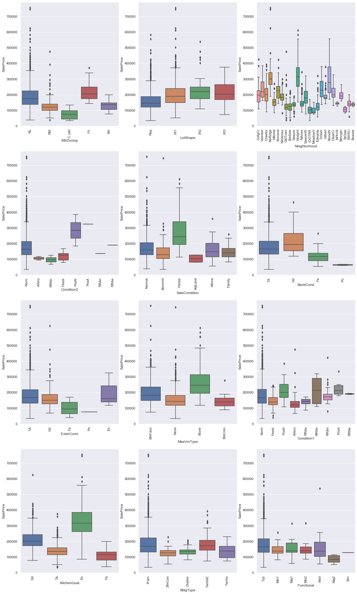
Boxplots are a great way to give a clear and precise overview of our categorical values. Overall, notice that most of the plots have a fairly normal distribution, however, there are lots of outliers, with high standard deviation and variance present. The box plots are also short (except Neighborhood) which implies that the data points are similar and in short range. From the first plot, the zoning category with the highest price average is the floating village residential; the neighborhood with the most expensive houses are Northridge Heights, Northridge and Stone Brook; From condition1, proximity to the park (PosN) is positively correlated to price of house; In exterCond, excellent exterior materials are more dispersed after 150,000; Excellent kitchen qualities have an interquartile range of approximately 250,000 and 400,000.

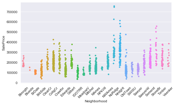
#let us look at neighborhood more closely
plt.figure(figsize=(9,5))
sns.stripplot(x = train_df.Neighborhood, y = train_df.SalePrice,
              order = np.sort(train_df.Neighborhood.unique()),
              alpha=1)

plt.xticks(rotation=45)
plt.show()

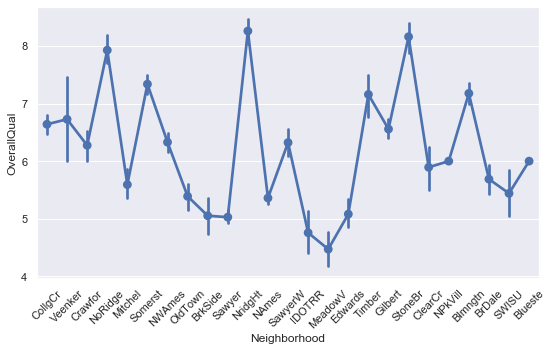
#Neughborhood vs Overall Quality
plt.figure(figsize=(9,5))
sns.pointplot(x = train_df.Neighborhood, y = train_df.OverallQual)
plt.xticks(rotation=45)
plt.show()

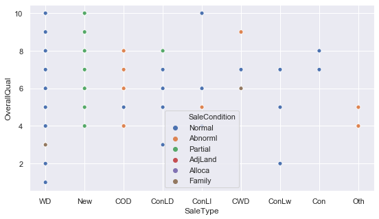
#compare SalePrice and SaleType with respect to SaleCondition
plt.figure(figsize=(9,5))
sns.scatterplot(x="SaleType",y="OverallQual",
                hue="SaleCondition",data=train_df)

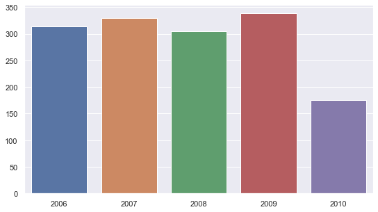
#What are the number of houses sold per year
year_count = train_df.YrSold.value_counts()
plt.figure(figsize= (9, 5))
sns.barplot(year_count.index, year_count.values, alpha=1)
plt.show()

4. Prepare Data for Machine Learning Algorithms.

This stage involves data cleaning, wrangling and feature engineering. This prepares the data in a the best possible way that it can be accepted by ML models.

4.1. General Tidying

data = pd.concat([train_df, test_df])

data["MSSubClass"] = data["MSSubClass"].astype(str) #Find variables in wrong types. MSSubClass is ordinal, and not an int.

data.info()

<class 'pandas.core.frame.DataFrame'>
Int64Index: 2919 entries, 0 to 1458
Data columns (total 81 columns):
 #   Column         Non-Null Count  Dtype  
---  ------         --------------  -----  
 0   Id             2919 non-null   int64  
 1   MSSubClass     2919 non-null   object
 2   MSZoning       2915 non-null   object
 3   LotFrontage    2433 non-null   float64
 4   LotArea        2919 non-null   int64  
 5   Street         2919 non-null   object
 6   Alley          198 non-null    object
 7   LotShape       2919 non-null   object
 8   LandContour    2919 non-null   object
 9   Utilities      2917 non-null   object
 10  LotConfig      2919 non-null   object
 11  LandSlope      2919 non-null   object
 12  Neighborhood   2919 non-null   object
 13  Condition1     2919 non-null   object
 14  Condition2     2919 non-null   object
 15  BldgType       2919 non-null   object
 16  HouseStyle     2919 non-null   object
 17  OverallQual    2919 non-null   int64  
 18  OverallCond    2919 non-null   int64  
 19  YearBuilt      2919 non-null   int64  
 20  YearRemodAdd   2919 non-null   int64  
 21  RoofStyle      2919 non-null   object
 22  RoofMatl       2919 non-null   object
 23  Exterior1st    2918 non-null   object
 24  Exterior2nd    2918 non-null   object
 25  MasVnrType     2895 non-null   object
 26  MasVnrArea     2896 non-null   float64
 27  ExterQual      2919 non-null   object
 28  ExterCond      2919 non-null   object
 29  Foundation     2919 non-null   object
 30  BsmtQual       2838 non-null   object
 31  BsmtCond       2837 non-null   object
 32  BsmtExposure   2837 non-null   object
 33  BsmtFinType1   2840 non-null   object
 34  BsmtFinSF1     2918 non-null   float64
 35  BsmtFinType2   2839 non-null   object
 36  BsmtFinSF2     2918 non-null   float64
 37  BsmtUnfSF      2918 non-null   float64
 38  TotalBsmtSF    2918 non-null   float64
 39  Heating        2919 non-null   object
 40  HeatingQC      2919 non-null   object
 41  CentralAir     2919 non-null   object
 42  Electrical     2918 non-null   object
 43  1stFlrSF       2919 non-null   int64  
 44  2ndFlrSF       2919 non-null   int64  
 45  LowQualFinSF   2919 non-null   int64  
 46  GrLivArea      2919 non-null   int64  
 47  BsmtFullBath   2917 non-null   float64
 48  BsmtHalfBath   2917 non-null   float64
 49  FullBath       2919 non-null   int64  
 50  HalfBath       2919 non-null   int64  
 51  BedroomAbvGr   2919 non-null   int64  
 52  KitchenAbvGr   2919 non-null   int64  
 53  KitchenQual    2918 non-null   object
 54  TotRmsAbvGrd   2919 non-null   int64  
 55  Functional     2917 non-null   object
 56  Fireplaces     2919 non-null   int64  
 57  FireplaceQu    1499 non-null   object
 58  GarageType     2762 non-null   object
 59  GarageYrBlt    2760 non-null   float64
 60  GarageFinish   2760 non-null   object
 61  GarageCars     2918 non-null   float64
 62  GarageArea     2918 non-null   float64
 63  GarageQual     2760 non-null   object
 64  GarageCond     2760 non-null   object
 65  PavedDrive     2919 non-null   object
 66  WoodDeckSF     2919 non-null   int64  
 67  OpenPorchSF    2919 non-null   int64  
 68  EnclosedPorch  2919 non-null   int64  
 69  3SsnPorch      2919 non-null   int64  
 70  ScreenPorch    2919 non-null   int64  
 71  PoolArea       2919 non-null   int64  
 72  PoolQC         10 non-null     object
 73  Fence          571 non-null    object
 74  MiscFeature    105 non-null    object
 75  MiscVal        2919 non-null   int64  
 76  MoSold         2919 non-null   int64  
 77  YrSold         2919 non-null   int64  
 78  SaleType       2918 non-null   object
 79  SaleCondition  2919 non-null   object
 80  SalePrice      1460 non-null   float64
dtypes: float64(12), int64(25), object(44)
memory usage: 1.8+ MB

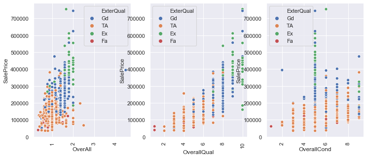
4.2. Feature Extraction

#Try out attribute combination
data["OverAll"] = data["OverallQual"] / data["OverallCond"]


data["AgeSold"] = data["YrSold"] - data["YearBuilt"]


data["TotalBsmt"] = data["BsmtFinSF2"] + data["BsmtFinSF1"]


data["TotalBath"] = data["FullBath"] + data["HalfBath"] *0.5

data["OverAll"] = data["OverallQual"] / data["OverallCond"]

attr_combo1 = ["OverAll", "OverallQual", "OverallCond"]
fig, ax = plt.subplots(1, 3, figsize=(12, 5))
for var, subplot in zip(attr_combo1, ax.flatten()):
    sns.scatterplot(x=var, y='SalePrice' , hue="ExterQual", data=data, ax=subplot)
    for label in subplot.get_xticklabels():
        label.set_rotation(90)

4.3. Checking for missing values and Dropping irrelevant Faetures

#First lets see how many missing values per attribute
null = data.isnull().sum().sort_values(ascending=False)
null[null>0]

PoolQC          2909
MiscFeature     2814
Alley           2721
Fence           2348
SalePrice       1459
FireplaceQu     1420
LotFrontage      486
GarageQual       159
GarageYrBlt      159
GarageFinish     159
GarageCond       159
GarageType       157
BsmtCond          82
BsmtExposure      82
BsmtQual          81
BsmtFinType2      80
BsmtFinType1      79
MasVnrType        24
MasVnrArea        23
MSZoning           4
Functional         2
BsmtFullBath       2
Utilities          2
BsmtHalfBath       2
KitchenQual        1
Exterior2nd        1
TotalBsmt          1
Exterior1st        1
Electrical         1
GarageCars         1
GarageArea         1
BsmtUnfSF          1
BsmtFinSF2         1
BsmtFinSF1         1
SaleType           1
TotalBsmtSF        1
dtype: int64

def corr_(data):
    correlation = data.corr()

    fig, ax = plt.subplots(figsize=(30,20))
    sns.heatmap(correlation, vmax=1.0, center=0, fmt='.2f', square=True,
               linewidth=.5, annot=True, cbar_kws={'shrink': .70})

    plt.show()

corr_(data)

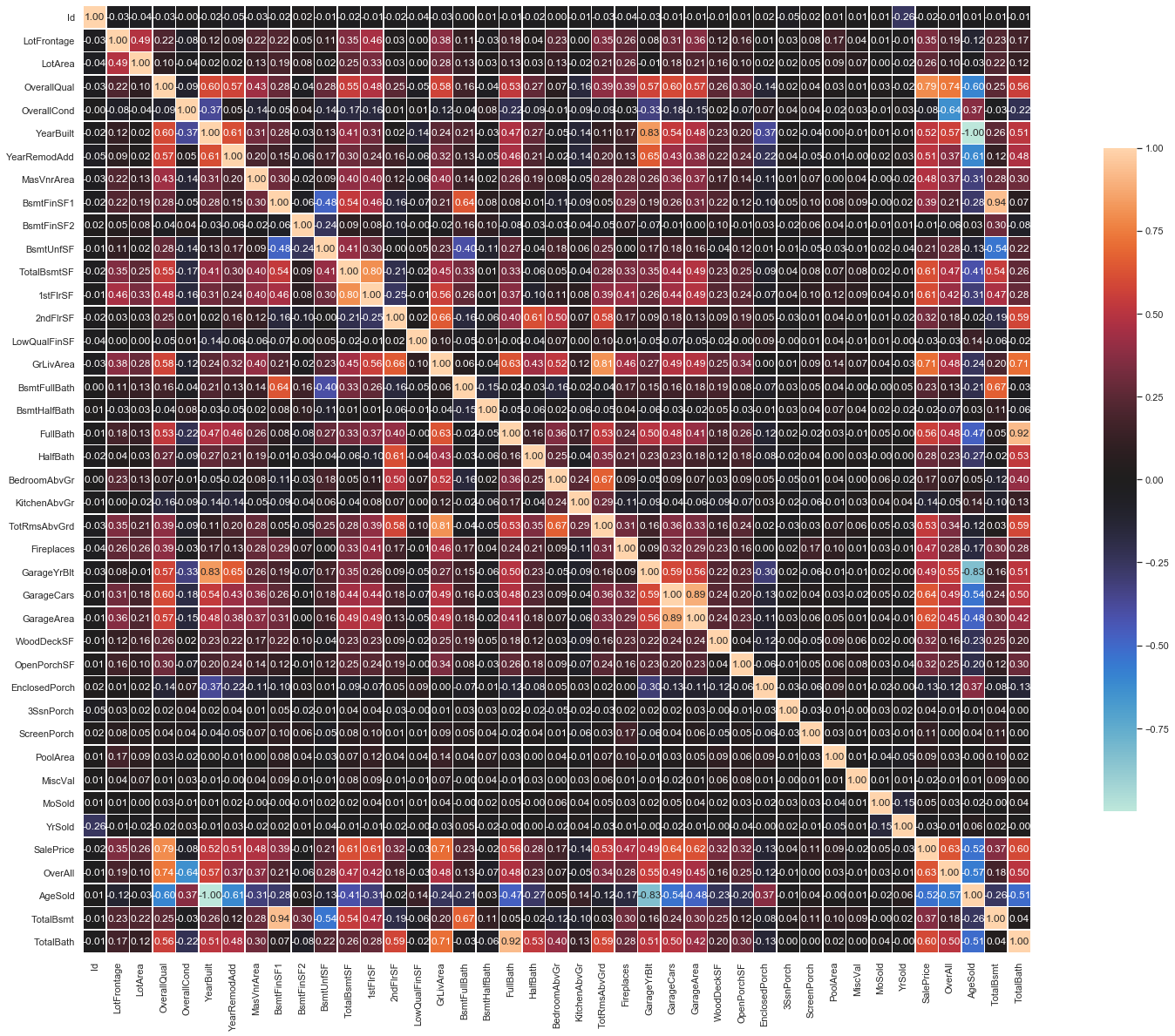
# I think the features with high missing values are unavailable not missing (Note the differece). Eg, there are no pools in
# almost all the houses. For this reason, we will not drop any variable with missing instances but fill them. However, we will
# drop multicollinear predictors with a threashold of [-7,7].

data = data.drop(['Id', 'SalePrice'], axis=1).copy()
data = data.drop(['1stFlrSF', 'TotalBsmt', 'FullBath', 'OverAll', 'AgeSold'], axis=1) #from correlation
data = data.drop(['Utilities', 'Street', 'PoolQC', 'MiscFeature', 'HalfBath', 'LowQualFinSF', 'GarageQual', '3SsnPorch'], axis=1)

4.4. Feature Transform

train = data.iloc[:1460]
test = data.iloc[1460:]

train.sample(5)

	MSSubClass	MSZoning	LotFrontage	LotArea	Alley	LotShape	LandContour	LotConfig	LandSlope	Neighborhood	Condition1	Condition2	BldgType	HouseStyle	OverallQual	OverallCond	YearBuilt	YearRemodAdd	RoofStyle	RoofMatl	Exterior1st	Exterior2nd	MasVnrType	MasVnrArea	ExterQual	ExterCond	Foundation	BsmtQual	BsmtCond	BsmtExposure	BsmtFinType1	BsmtFinSF1	BsmtFinType2	BsmtFinSF2	BsmtUnfSF	TotalBsmtSF	Heating	HeatingQC	CentralAir	Electrical	2ndFlrSF	GrLivArea	BsmtFullBath	BsmtHalfBath	BedroomAbvGr	KitchenAbvGr	KitchenQual	TotRmsAbvGrd	Functional	Fireplaces	FireplaceQu	GarageType	GarageYrBlt	GarageFinish	GarageCars	GarageArea	GarageCond	PavedDrive	WoodDeckSF	OpenPorchSF	EnclosedPorch	ScreenPorch	PoolArea	Fence	MiscVal	MoSold	YrSold	SaleType	SaleCondition	TotalBath
694	50	RM	51.0	6120	NaN	Reg	Lvl	Corner	Gtl	BrkSide	Norm	Norm	1Fam	1.5Fin	5	6	1936	1950	Gable	CompShg	Wd Sdng	Wd Sdng	None	0.0	TA	Fa	BrkTil	TA	TA	No	Unf	0.0	Unf	0.0	927.0	927.0	GasA	TA	Y	SBrkr	472	1539	0.0	0.0	3	1	TA	5	Typ	0	NaN	Detchd	1995.0	Unf	2.0	576.0	TA	Y	112	0	0	0	0	MnPrv	0	4	2009	WD	Normal	1.5
908	20	RL	NaN	8885	NaN	IR1	Low	Inside	Mod	Mitchel	Norm	Norm	1Fam	1Story	5	5	1983	1983	Gable	CompShg	HdBoard	HdBoard	None	0.0	TA	TA	CBlock	Gd	TA	Av	BLQ	301.0	ALQ	324.0	239.0	864.0	GasA	TA	Y	SBrkr	0	902	1.0	0.0	2	1	TA	5	Typ	0	NaN	Attchd	1983.0	Unf	2.0	484.0	TA	Y	164	0	0	0	0	MnPrv	0	6	2006	WD	Normal	1.0
381	20	FV	60.0	7200	Pave	Reg	Lvl	Inside	Gtl	Somerst	Norm	Norm	1Fam	1Story	7	5	2006	2006	Gable	CompShg	VinylSd	VinylSd	None	0.0	Gd	TA	PConc	Gd	Gd	No	Unf	0.0	Unf	0.0	1293.0	1293.0	GasA	Ex	Y	SBrkr	0	1301	1.0	0.0	2	1	Gd	5	Typ	1	Gd	Attchd	2006.0	RFn	2.0	572.0	TA	Y	216	121	0	0	0	NaN	0	8	2006	New	Partial	2.0
341	20	RH	60.0	8400	NaN	Reg	Lvl	Inside	Gtl	SawyerW	Feedr	Norm	1Fam	1Story	4	4	1950	1950	Gable	CompShg	Wd Sdng	AsbShng	None	0.0	Fa	Fa	CBlock	TA	Fa	No	Unf	0.0	Unf	0.0	721.0	721.0	GasA	Gd	Y	SBrkr	0	841	0.0	0.0	2	1	TA	4	Typ	0	NaN	CarPort	1950.0	Unf	1.0	294.0	TA	N	250	0	24	0	0	NaN	0	9	2009	WD	Normal	1.0
796	20	RL	71.0	8197	NaN	Reg	Lvl	Inside	Gtl	Sawyer	Norm	Norm	1Fam	1Story	6	5	1977	1977	Gable	CompShg	Plywood	Plywood	BrkFace	148.0	TA	TA	CBlock	TA	TA	No	Unf	0.0	Unf	0.0	660.0	660.0	GasA	Ex	Y	SBrkr	0	1285	0.0	0.0	3	1	TA	7	Typ	1	TA	Attchd	1977.0	RFn	2.0	528.0	TA	Y	138	0	0	0	0	MnPrv	0	4	2007	WD	Normal	1.5

train_num = train.select_dtypes(include=[np.number])#select all numeric columns
train_num.head()

	LotFrontage	LotArea	OverallQual	OverallCond	YearBuilt	YearRemodAdd	MasVnrArea	BsmtFinSF1	BsmtFinSF2	BsmtUnfSF	TotalBsmtSF	2ndFlrSF	GrLivArea	BsmtFullBath	BsmtHalfBath	BedroomAbvGr	KitchenAbvGr	TotRmsAbvGrd	Fireplaces	GarageYrBlt	GarageCars	GarageArea	WoodDeckSF	OpenPorchSF	EnclosedPorch	ScreenPorch	PoolArea	MiscVal	MoSold	YrSold	TotalBath
0	65.0	8450	7	5	2003	2003	196.0	706.0	0.0	150.0	856.0	854	1710	1.0	0.0	3	1	8	0	2003.0	2.0	548.0	0	61	0	0	0	0	2	2008	2.5
1	80.0	9600	6	8	1976	1976	0.0	978.0	0.0	284.0	1262.0	0	1262	0.0	1.0	3	1	6	1	1976.0	2.0	460.0	298	0	0	0	0	0	5	2007	2.0
2	68.0	11250	7	5	2001	2002	162.0	486.0	0.0	434.0	920.0	866	1786	1.0	0.0	3	1	6	1	2001.0	2.0	608.0	0	42	0	0	0	0	9	2008	2.5
3	60.0	9550	7	5	1915	1970	0.0	216.0	0.0	540.0	756.0	756	1717	1.0	0.0	3	1	7	1	1998.0	3.0	642.0	0	35	272	0	0	0	2	2006	1.0
4	84.0	14260	8	5	2000	2000	350.0	655.0	0.0	490.0	1145.0	1053	2198	1.0	0.0	4	1	9	1	2000.0	3.0	836.0	192	84	0	0	0	0	12	2008	2.5

from sklearn.pipeline import Pipeline as pl
from sklearn.impute import SimpleImputer as si
from sklearn.preprocessing import RobustScaler as rs

num_pipeline = pl([
    ('imputer', si(strategy="mean")),
    ('scaler', rs()),
    ])

train_num_trx = num_pipeline.fit_transform(train_num)
print(train_num_trx)
print('***' * 30)
print(train_num_trx.shape)
print('***' * 30)
print(np.isnan(train_num_trx).sum())

[[-0.26578728 -0.25407609  0.5        ... -1.33333333  0.
   0.33333333]
 [ 0.5236864   0.03001482  0.         ... -0.33333333 -0.5
   0.        ]
 [-0.10789255  0.43762352  0.5        ...  1.          0.
   0.33333333]
 ...
 [-0.2131557  -0.10783103  0.5        ... -0.33333333  1.
   0.        ]
 [-0.10789255  0.05891798 -0.5        ... -0.66666667  1.
  -0.66666667]
 [ 0.26052851  0.11326581 -0.5        ...  0.          0.
  -0.33333333]]
******************************************************************************************
(1460, 31)
******************************************************************************************
0

Non numeric Pipeline

train_ordinal = train.select_dtypes(exclude=[np.number])
train_ordinal.head()

	MSSubClass	MSZoning	Alley	LotShape	LandContour	LotConfig	LandSlope	Neighborhood	Condition1	Condition2	BldgType	HouseStyle	RoofStyle	RoofMatl	Exterior1st	Exterior2nd	MasVnrType	ExterQual	ExterCond	Foundation	BsmtQual	BsmtCond	BsmtExposure	BsmtFinType1	BsmtFinType2	Heating	HeatingQC	CentralAir	Electrical	KitchenQual	Functional	FireplaceQu	GarageType	GarageFinish	GarageCond	PavedDrive	Fence	SaleType	SaleCondition
0	60	RL	NaN	Reg	Lvl	Inside	Gtl	CollgCr	Norm	Norm	1Fam	2Story	Gable	CompShg	VinylSd	VinylSd	BrkFace	Gd	TA	PConc	Gd	TA	No	GLQ	Unf	GasA	Ex	Y	SBrkr	Gd	Typ	NaN	Attchd	RFn	TA	Y	NaN	WD	Normal
1	20	RL	NaN	Reg	Lvl	FR2	Gtl	Veenker	Feedr	Norm	1Fam	1Story	Gable	CompShg	MetalSd	MetalSd	None	TA	TA	CBlock	Gd	TA	Gd	ALQ	Unf	GasA	Ex	Y	SBrkr	TA	Typ	TA	Attchd	RFn	TA	Y	NaN	WD	Normal
2	60	RL	NaN	IR1	Lvl	Inside	Gtl	CollgCr	Norm	Norm	1Fam	2Story	Gable	CompShg	VinylSd	VinylSd	BrkFace	Gd	TA	PConc	Gd	TA	Mn	GLQ	Unf	GasA	Ex	Y	SBrkr	Gd	Typ	TA	Attchd	RFn	TA	Y	NaN	WD	Normal
3	70	RL	NaN	IR1	Lvl	Corner	Gtl	Crawfor	Norm	Norm	1Fam	2Story	Gable	CompShg	Wd Sdng	Wd Shng	None	TA	TA	BrkTil	TA	Gd	No	ALQ	Unf	GasA	Gd	Y	SBrkr	Gd	Typ	Gd	Detchd	Unf	TA	Y	NaN	WD	Abnorml
4	60	RL	NaN	IR1	Lvl	FR2	Gtl	NoRidge	Norm	Norm	1Fam	2Story	Gable	CompShg	VinylSd	VinylSd	BrkFace	Gd	TA	PConc	Gd	TA	Av	GLQ	Unf	GasA	Ex	Y	SBrkr	Gd	Typ	TA	Attchd	RFn	TA	Y	NaN	WD	Normal

 import category_encoders as ce

ordinal_pipeline = pl([
    ('imputer', si(strategy="most_frequent", fill_value='None')),
    ('ord_encoder', ce.OrdinalEncoder(return_df=False)),
    ('scaler', rs()),
])

train_ord_trx = ordinal_pipeline.fit_transform(train_ordinal)  
print(train_ord_trx)
print('***' * 30)
print(train_ord_trx.shape)
print('***' * 30)
print(np.isnan(train_ord_trx).sum())

[[ 0.2  0.   0.  ...  0.   0.   0. ]
 [-0.6  0.   0.  ...  0.   0.   0. ]
 [ 0.2  0.   0.  ...  0.   0.   0. ]
 ...
 [ 0.4  0.   0.  ...  2.   0.   0. ]
 [-0.6  0.   0.  ...  0.   0.   0. ]
 [-0.6  0.   0.  ...  0.   0.   0. ]]
******************************************************************************************
(1460, 39)
******************************************************************************************
0

#combine numerical and categorical pipelines
from sklearn.compose import ColumnTransformer as colt

num_attribs = list(train_num)
#nom_attribs = list(train_nominal)
ord_attribs = list(train_ordinal)


full_pipeline = colt([
    ("num", num_pipeline, num_attribs),
   # ("nom", nominal_pipeline, nom_attribs),
    ("ord", ordinal_pipeline, ord_attribs)
])

X_train = full_pipeline.fit_transform(train)
X_test = full_pipeline.transform(test)

Recheck and Rename

print(X_train.shape)
print(X_test.shape)

(1460, 70)
(1459, 70)

#To reduce the distance between values, such that a slght change in x affects y.
y = np.log1p(train_df['SalePrice']).copy()
y_test = np.log1p(sub_df['SalePrice']).copy()

5.0. Select and Train a Model

from sklearn.linear_model import LinearRegression
from sklearn.ensemble import RandomForestRegressor
from sklearn.linear_model import Lasso
import xgboost as xgb
from sklearn.linear_model import Ridge
from sklearn.svm import SVR
from sklearn.neighbors import KNeighborsRegressor

from sklearn.metrics import mean_squared_error as mse
from sklearn.metrics import mean_absolute_error as mae

linear = LinearRegression()
linear.fit(X_train, y)
linear_predict = linear.predict(X_test)
linear_predict

array([11.61963892, 11.93880308, 12.04341483, ..., 12.05827928,
       11.69047332, 12.42217636])

#We can see the actual values and make visual comparisons

print("Top 3 Labels:", list(y_test.head(3)))
print("Last 3 Labels:", list(y_test.tail(3)))

Top 3 Labels: [12.039297922968691, 12.142916602935376, 12.120431330864875]
Last 3 Labels: [12.297846686923938, 12.127707128738267, 12.142828575069593]

lr_mse = mse(linear_predict, y_test)
lr_rmse = np.sqrt(lr_mse)
lr_rmse

0.37529958427243454

forest = RandomForestRegressor(n_estimators=500, random_state=42)
forest.fit(X_train, y)
forest_predict = forest.predict(X_test)
forest_predict

array([11.73574016, 11.94428311, 12.08468668, ..., 11.94771477,
       11.66495922, 12.37360112])

rfr_mse = mse(forest_predict, y_test)
rfr_rmse = np.sqrt(rfr_mse)
rfr_rmse

0.3639948694315479

lasso = Lasso(max_iter=1000, alpha=0.01)
lasso.fit(X_train, y)
lasso_pred = lasso.predict(X_test)
lasso_pred

array([11.73449396, 11.88775546, 12.05602704, ..., 12.02604719,
       11.6888728 , 12.38120214])

lasso_mse = mse(lasso_pred, y_test)
lasso_rmse = np.sqrt(lasso_mse)
lasso_rmse

0.3458549542156051

train_matrix = xgb.DMatrix(X_train, y)
test_matrix = xgb.DMatrix(X_test)

xg = xgb.XGBRegressor(objective='reg:squarederror', n_estimators=500,
         random_state=42)
xg .fit(X_train, y)
xg_pred = xg.predict(X_test)
xg_pred

array([11.706657, 11.984388, 12.152975, ..., 12.082707, 11.706811,
       12.328882], dtype=float32)

xg_mse = mse(xg_pred, y_test)
xg_rmse = np.sqrt(xg_mse)
xg_rmse

0.3848714208977196

ridge = Ridge()
ridge.fit(X_train, y)
ridge_pred = ridge.predict(X_test)
ridge_pred

array([11.62101732, 11.94041983, 12.0437113 , ..., 12.05949654,
       11.69001701, 12.42200935])

ridge_mse = mse(ridge_pred, y_test)
ridge_rmse = np.sqrt(ridge_mse)
ridge_rmse

0.37495026973019624

svm = SVR()
svm.fit(X_train, y)
svm_pred = svm.predict(X_test)
svm_pred

array([11.97421201, 12.25842922, 12.0408935 , ..., 12.04879778,
       11.87755258, 12.05781983])

svm_mse = mse(svm_pred, y_test)
svm_rmse = np.sqrt(svm_mse)
svm_rmse

0.1559147202143059

knn = KNeighborsRegressor(n_neighbors=3)
knn.fit(X_train, y)
knn_pred = knn.predict(X_test)
knn_pred

array([11.84492742, 11.66607959, 12.13417428, ..., 11.86700169,
       11.9627464 , 12.30373907])

knn_mse = mse(knn_pred, y_test)
knn_rmse = np.sqrt(knn_mse)
knn_rmse

0.32369617565934844

Our support vector regressor outperforms the others by a mile. It is efinitely overfitting. For practice, fine-tune the other regressors and compare how they perform.

Validating & Fine-Tuning Model

We now have some promising models–random forest and xgboost. Next step is to fine-tune and validate them. Notice in the models above, we have placed the barest of parameters. This is beacuse there is no human way to exaustively find the best combinations of hyperparameters for our choosen model. Think of it as tuning a radio nob to find the clearest station. Thanks to scikitlearn’s GridSearchCV and RandomisedSearchCV, we can do this automatically.

from sklearn.model_selection import RandomizedSearchCV
from scipy.stats import randint, uniform

xgb_regg = xgb.XGBRegressor(objective='reg:squarederror', random_state=42)

params_xgb = {
        'max_depth': [3, 4, 5, 6, 7],
        'num_boost_round': [10, 25],
        'subsample': [0.9, 1.0],
        'colsample_bytree': [0.4, 0.5, 0.6],
        'colsample_bylevel': [0.4, 0.5, 0.6],
        'min_child_weight': [1.0, 3.0],
        'gamma': [0, 0.25],
       'reg_lambda': [1.0, 5.0, 7.0],
        'n_estimators': randint(200, 2000)
        }

random_ = RandomizedSearchCV(xgb_regg, param_distributions=params_xgb, n_iter=20, cv=5,
         scoring='neg_mean_squared_error', n_jobs=1,  random_state=42)

random_.fit(X_train, y)

RandomizedSearchCV(cv=5, error_score=nan,
                   estimator=XGBRegressor(base_score=0.5, booster='gbtree',
                                          colsample_bylevel=1,
                                          colsample_bynode=1,
                                          colsample_bytree=1, gamma=0,
                                          importance_type='gain',
                                          learning_rate=0.1, max_delta_step=0,
                                          max_depth=3, min_child_weight=1,
                                          missing=None, n_estimators=100,
                                          n_jobs=1, nthread=None,
                                          objective='reg:squarederror',
                                          random_state=42, reg...
                                        'gamma': [0, 0.25],
                                        'max_depth': [3, 4, 5, 6, 7],
                                        'min_child_weight': [1.0, 3.0],
                                        'n_estimators': <scipy.stats._distn_infrastructure.rv_frozen object at 0x0000022AC8AB1748>,
                                        'num_boost_round': [10, 25],
                                        'reg_lambda': [1.0, 5.0, 7.0],
                                        'subsample': [0.9, 1.0]},
                   pre_dispatch='2*n_jobs', random_state=42, refit=True,
                   return_train_score=False, scoring='neg_mean_squared_error',
                   verbose=0)

random_.best_params_

{'colsample_bylevel': 0.4,
 'colsample_bytree': 0.4,
 'gamma': 0,
 'max_depth': 3,
 'min_child_weight': 3.0,
 'n_estimators': 1352,
 'num_boost_round': 25,
 'reg_lambda': 7.0,
 'subsample': 0.9}

 random_.best_estimator_

XGBRegressor(base_score=0.5, booster='gbtree', colsample_bylevel=0.4,
             colsample_bynode=1, colsample_bytree=0.4, gamma=0,
             importance_type='gain', learning_rate=0.1, max_delta_step=0,
             max_depth=3, min_child_weight=3.0, missing=None, n_estimators=1352,
             n_jobs=1, nthread=None, num_boost_round=25,
             objective='reg:squarederror', random_state=42, reg_alpha=0,
             reg_lambda=7.0, scale_pos_weight=1, seed=None, silent=None,
             subsample=0.9, verbosity=1)

model = random_.best_estimator_

pred2 = model.predict(X_test)

prediction2 = np.expm1(pred2)
output2 = pd.DataFrame({'Id':test_df.Id, 'SalePrice':prediction2})
output2.head()

	Id	SalePrice
0	1461	118886.632812
1	1462	161320.671875
2	1463	187420.640625
3	1464	192596.515625
4	1465	181116.140625

output2.to_csv('xgb8.csv', index=False)

feature_importance = random_.best_estimator_.feature_importances_
attributes = num_attribs + ord_attribs
sorted(zip(feature_importance, attributes), reverse=True)

[(0.17045057, 'OverallQual'),
 (0.15516618, 'GarageCars'),
 (0.07165706, 'Fireplaces'),
 (0.047740616, 'TotalBath'),
 (0.044116538, 'CentralAir'),
 (0.042846948, 'GrLivArea'),
 (0.029083796, 'YearRemodAdd'),
 (0.026234755, 'GarageArea'),
 (0.026158102, 'YearBuilt'),
 (0.025795698, 'TotalBsmtSF'),
 (0.02197889, 'OverallCond'),
 (0.020921756, 'GarageYrBlt'),
 (0.016097259, 'BsmtFinSF1'),
 (0.016042368, 'BsmtFinType1'),
 (0.015377405, 'KitchenAbvGr'),
 (0.014440038, 'Functional'),
 (0.013417843, 'GarageFinish'),
 (0.013118019, 'MSZoning'),
 (0.012961783, '2ndFlrSF'),
 (0.011720444, 'Condition2'),
 (0.011579358, 'BsmtQual'),
 (0.0094911475, 'BsmtExposure'),
 (0.008285343, 'BldgType'),
 (0.007862613, 'Foundation'),
 (0.0077409633, 'KitchenQual'),
 (0.007587692, 'LotArea'),
 (0.0071345335, 'PavedDrive'),
 (0.0067442725, 'LotFrontage'),
 (0.0063789533, 'BsmtFullBath'),
 (0.006071903, 'Condition1'),
 (0.00599091, 'Fence'),
 (0.0058421427, 'TotRmsAbvGrd'),
 (0.0053032683, 'MiscVal'),
 (0.0052680154, 'Neighborhood'),
 (0.0052600936, 'PoolArea'),
 (0.0052061058, 'ScreenPorch'),
 (0.0051219543, 'SaleCondition'),
 (0.0048817596, 'OpenPorchSF'),
 (0.004331854, 'ExterQual'),
 (0.0039200904, 'RoofMatl'),
 (0.003806459, 'ExterCond'),
 (0.0036296323, 'LotShape'),
 (0.0036123004, 'WoodDeckSF'),
 (0.0034323013, 'BsmtFinSF2'),
 (0.003272554, 'HeatingQC'),
 (0.0032045993, 'Exterior1st'),
 (0.0030321914, 'BedroomAbvGr'),
 (0.003013601, 'HouseStyle'),
 (0.0029762562, 'GarageType'),
 (0.0027719024, 'MSSubClass'),
 (0.0027711922, 'MoSold'),
 (0.002718122, 'SaleType'),
 (0.002393617, 'GarageCond'),
 (0.0023310797, 'Exterior2nd'),
 (0.0023181213, 'YrSold'),
 (0.002283722, 'BsmtFinType2'),
 (0.002270854, 'BsmtCond'),
 (0.0021721106, 'EnclosedPorch'),
 (0.0021401297, 'MasVnrType'),
 (0.0021189386, 'MasVnrArea'),
 (0.0020685012, 'LotConfig'),
 (0.0020539796, 'FireplaceQu'),
 (0.0020457623, 'Heating'),
 (0.0020246482, 'BsmtUnfSF'),
 (0.0019086191, 'RoofStyle'),
 (0.001887537, 'Electrical'),
 (0.0018400064, 'LandSlope'),
 (0.0017197807, 'LandContour'),
 (0.001689854, 'Alley'),
 (0.0011625615, 'BsmtHalfBath')]