
Classification in View: Iris Dataset
1. Introduction
Explaining how a model works to non science people is one of the most basic yet critical aspects of a data scientist. You build a model which is giving you pretty impressive results, but what was the process behind it? As a data scientist, you need to have answers to often asked questions behind the reasoning in machine learning algorithms. This notebook describes processes behind some of the popular classification models used in data science today. They include; K-Nearest Neighbour, Logistic regression, support vector machine, Decision trees and some popular Ensemble methods.
“If you can’t explain it simply, you don’t understand it well enough”. Albert Einstein
In our introductory post, we discussed the difference between prediction and classification. That all supervised learning problems are predictive in nature, including predicting continuous values and labels. However, we also noted that classification problems only deals with labels or classes as a response variable. In our last post, we thoughrouly dealt with predicting the price of diamonds with Linear Regression, we saw how gradient descent works, we explained the tradeoff between Bias and Variance and also explained how they may be solved with regularisation techniques.
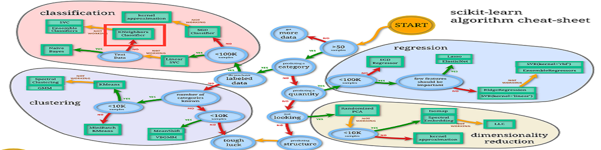
In this post, We will be using a simple, yet popular multi-class labeled dataset -Iris to understand the logics of classification algorithms. We are using the Iris dataset because it is easy to understand, plus it does not need to be cleaned so we can get into the nitty gritty of modelling as soon as possible. You can download the UCI dataset and get a description from Kaggle.. Also, this notebook only interprets mathematical deductions, not its derivations. However, links will be provided for further studies on how selected algorithm’s mathematical derivations are achieved. Without further ado, lets dive in.
#Import important libraries from python
import numpy as np
import pandas as pd
import matplotlib.pyplot as plt
%matplotlib inline
import seaborn as sns
#Load and view iris
iris = pd.read_csv('iris.csv')
iris.head(10)
| Id | SepalLengthCm | SepalWidthCm | PetalLengthCm | PetalWidthCm | Species | |
|---|---|---|---|---|---|---|
| 0 | 1 | 5.1 | 3.5 | 1.4 | 0.2 | Iris-setosa |
| 1 | 2 | 4.9 | 3.0 | 1.4 | 0.2 | Iris-setosa |
| 2 | 3 | 4.7 | 3.2 | 1.3 | 0.2 | Iris-setosa |
| 3 | 4 | 4.6 | 3.1 | 1.5 | 0.2 | Iris-setosa |
| 4 | 5 | 5.0 | 3.6 | 1.4 | 0.2 | Iris-setosa |
| 5 | 6 | 5.4 | 3.9 | 1.7 | 0.4 | Iris-setosa |
| 6 | 7 | 4.6 | 3.4 | 1.4 | 0.3 | Iris-setosa |
| 7 | 8 | 5.0 | 3.4 | 1.5 | 0.2 | Iris-setosa |
| 8 | 9 | 4.4 | 2.9 | 1.4 | 0.2 | Iris-setosa |
| 9 | 10 | 4.9 | 3.1 | 1.5 | 0.1 | Iris-setosa |
As you can see, there is an ‘Id’ column that we need to drop from the dataframe since it mimics the index
iris = iris.drop(['Id'], axis=1)
iris.info()
<class 'pandas.core.frame.DataFrame'>
RangeIndex: 150 entries, 0 to 149
Data columns (total 5 columns):
 #   Column         Non-Null Count  Dtype
---  ------         --------------  -----
 0   SepalLengthCm  150 non-null    float64
 1   SepalWidthCm   150 non-null    float64
 2   PetalLengthCm  150 non-null    float64
 3   PetalWidthCm   150 non-null    float64
 4   Species        150 non-null    object
dtypes: float64(4), object(1)
memory usage: 6.0+ KB
There are no null values in the dataset.
iris.describe() # Describes some statistical composition of the data
| SepalLengthCm | SepalWidthCm | PetalLengthCm | PetalWidthCm | |
|---|---|---|---|---|
| count | 150.000000 | 150.000000 | 150.000000 | 150.000000 |
| mean | 5.843333 | 3.054000 | 3.758667 | 1.198667 |
| std | 0.828066 | 0.433594 | 1.764420 | 0.763161 |
| min | 4.300000 | 2.000000 | 1.000000 | 0.100000 |
| 25% | 5.100000 | 2.800000 | 1.600000 | 0.300000 |
| 50% | 5.800000 | 3.000000 | 4.350000 | 1.300000 |
| 75% | 6.400000 | 3.300000 | 5.100000 | 1.800000 |
| max | 7.900000 | 4.400000 | 6.900000 | 2.500000 |
iris.Species.value_counts()
Iris-versicolor    50
Iris-setosa        50
Iris-virginica     50
Name: Species, dtype: int64
We have a perfectly balanced dataset.
Check what imbalanced dataset means
2. Some Visual Analysis
These colourful plots are gotten from seaborn library and pandas dataframe. They are also quite easy to use. Just a few lines of code and viola! Go through the features at Seaborn.org to help you start creating your own awesome plots.
### Boxplots displaying the range (min, quartiles and max) of a distribution.
iris.boxplot(by="Species", figsize=(15, 8)) #from pandas dataframe.boxplot
plt.show()
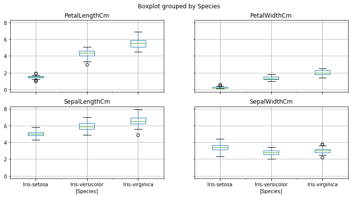
You can clearly see that iris-setosa’s petal length ranges from 1-2, max petal width of 1.8, average sepal length of 5cm and its 75th percentile is 3.8 of sepal width.
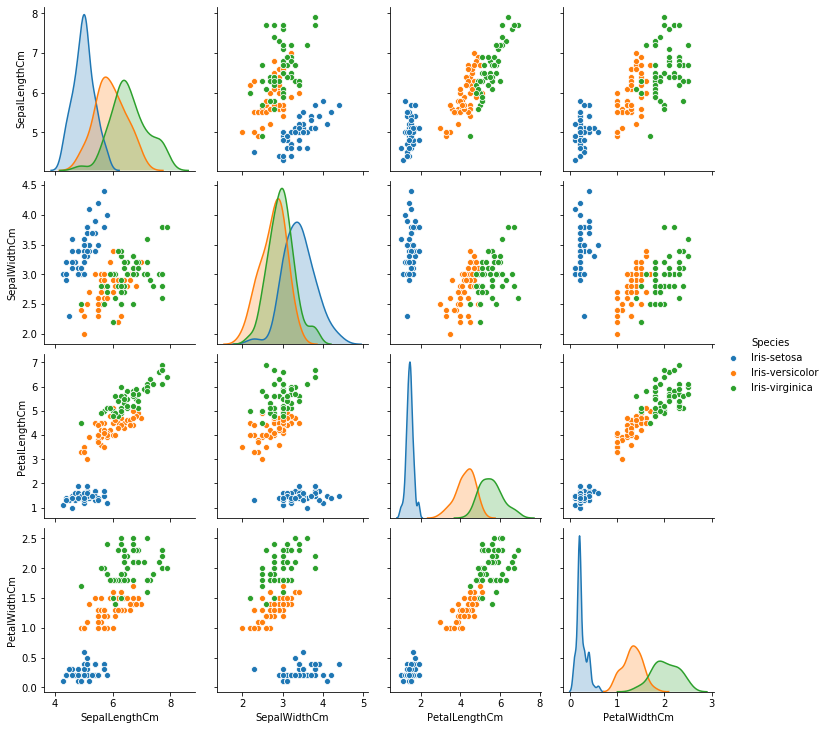
#Seaborn Pairplots showing all variables paired with all other variables
sns.pairplot(iris,hue='Species')
plt.show()
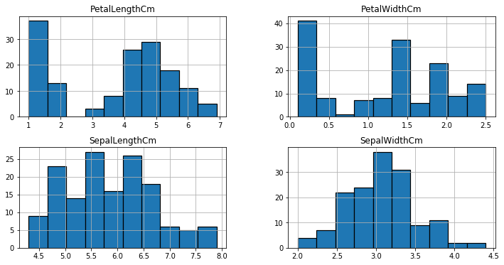
# Distribution plots from matplotlib.pyplot.gcf
iris.hist(edgecolor='black', linewidth=1.0)
fig=plt.gcf()
fig.set_size_inches(15,8)
3. Pre-Processing
# First, standardise numeric features especially for models that are sensitive to outliers.
# Next, use sklearn's label encoder to map 'Species' such that Iris-setosa=0, Iris-versicolor=1 and Iris-virginica=2

from sklearn.preprocessing import RobustScaler

train = iris.iloc[:, :4]#slice all rows and up to the 4th predictor
scaler = RobustScaler()

X = scaler.fit_transform(train)
X[:5]
array([[-0.53846154,  1.        , -0.84285714, -0.73333333],
       [-0.69230769,  0.        , -0.84285714, -0.73333333],
       [-0.84615385,  0.4       , -0.87142857, -0.73333333],
       [-0.92307692,  0.2       , -0.81428571, -0.73333333],
       [-0.61538462,  1.2       , -0.84285714, -0.73333333]])
from sklearn.preprocessing import LabelEncoder

target = iris['Species']
encoder =  LabelEncoder()
y = encoder.fit_transform(target)
y
array([0, 0, 0, 0, 0, 0, 0, 0, 0, 0, 0, 0, 0, 0, 0, 0, 0, 0, 0, 0, 0, 0,
       0, 0, 0, 0, 0, 0, 0, 0, 0, 0, 0, 0, 0, 0, 0, 0, 0, 0, 0, 0, 0, 0,
       0, 0, 0, 0, 0, 0, 1, 1, 1, 1, 1, 1, 1, 1, 1, 1, 1, 1, 1, 1, 1, 1,
       1, 1, 1, 1, 1, 1, 1, 1, 1, 1, 1, 1, 1, 1, 1, 1, 1, 1, 1, 1, 1, 1,
       1, 1, 1, 1, 1, 1, 1, 1, 1, 1, 1, 1, 2, 2, 2, 2, 2, 2, 2, 2, 2, 2,
       2, 2, 2, 2, 2, 2, 2, 2, 2, 2, 2, 2, 2, 2, 2, 2, 2, 2, 2, 2, 2, 2,
       2, 2, 2, 2, 2, 2, 2, 2, 2, 2, 2, 2, 2, 2, 2, 2, 2, 2])
# Now that we have X and y in good learning states, we can split dataset into train and test.
from sklearn.model_selection import train_test_split

X_train, X_test, y_train, y_test = train_test_split(X, y, test_size=0.2, random_state=0)
X_train.shape, X_test.shape
((120, 4), (30, 4))
4. Model Training
4.1. Logistic Regression.
Perequisite: Linear Regression.
In a lot of ways, linear regression and logistic regression are similar. However, one major difference is, where linear regression is used to predict continuous values, logistic regression is used for predicting classes. Logistic regression is a classification algorithm that predicts target variables in a Boolean order. That is, it askes the question, is a flower Iris-Setosa or not? Yes or No? True or False? (I am aware I am asking a question of a binary intuition while we have a multiclass dataset. Walk with me, we will address this shortly). Also, unlike linear regression that fits a line to the data, logistic regression fits an ‘S’ shaped logistic function - also called sigmoid function that can take any real-valued number and map it into a value between 0 and 1 as seen in the diagram below.
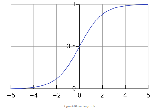
In other words, if the curve goes to positive infinity, y predicted will become 1, and if the curve goes to negative infinity, y predicted will become 0. One thing to note is, the sigmoid function with formula, 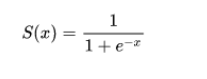 is responsible for estimating probabilities that squashes the predicted value into a range of (0, 1) since the numerator is always smaller than the denominator by 1. So far so good up until this point? Good! Now, lets see how a logistic regression model is trained.
This image from Experfy below does justice to visualise how logistic regression works.
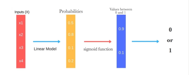
Just like a Linear Regression model, a Logistic Regression model computes a weighted sum of the input features (plus a bias term), but instead of outputting the result directly like the Linear Regression model does, it outputs the probabilities of the collection/sample of flowers given their sepal length, sepal width and so on… Then the sigmoid function groups each flower’s probability as a 0 or 1. For example, if the estimated probability that an iris flower-Iris-setosa is greater than 50%, then the model predicts that the flower belongs to that class (called the positive class, labeled “1”) otherwise it predicts that it does not (i.e., it belongs to the negative class, labeled “0”). If you want to understand the maths of it, you can head on to Christoph’s Page. He does a brilliant job at explaining its derivations as simple as possible. Remember how in Linear Regression you estimate the coefficients or weights and bias using ordinary least squares? Well, in Logistic Regression, we estimate the coefficients using Maximum Likelihood Estimation (MLE). The MLE is a “likelihood” maximization method, while OLS is a distance-minimizing approximation method. Have you noticed that Logistic Regression is a binary classifier yet? However, we have a multinomial classification task at hand. How can we solve this problem with Logistic Regression? One way is to use One-Vs-Rest algorithm. It basically trains the data as three separate binary classification problem. In its learning stage, One-Vs-Rest is implemented by training 3 logistic regression classifiers, one for each of the K classes (Iris-Setosa, Iris-Versicolor and Iris-Virginica) in the training dataset. When training the classifier for Iris-Setosa, it treats flowers 1-50 as +ve samples (y==1) and Iris-Versicolor and Iris-Virginica as -ve samples (y==0). When training the classifier for Class 2, we will treat flowers 51-100 as +ve samples (y==1) while Iris-Setosa and Iris-Virginica are treated as -ve samples (y==0). This will continue for all the classes. During prediction-One vs rest prediction of the test input, it computes the “probability” that it belongs to each class using the trained logistic regression classifiers. Your one-vs-rest prediction function will pick the class for which the corresponding logistic regression classifier outputs the highest probability and return the class label (1, 2,…, or K) as the prediction for the input example. Now that we understand the logic in Logistic Regression, we can use scikit-learn for training and prediction.
from sklearn.linear_model import LogisticRegression
from sklearn.metrics import classification_report
from sklearn.metrics import accuracy_score

log_clf = LogisticRegression(solver='lbfgs', max_iter=500,  multi_class='multinomial', penalty='none', random_state=0)
log_clf.fit(X_train, y_train)
LogisticRegression(C=1.0, class_weight=None, dual=False, fit_intercept=True,
                   intercept_scaling=1, l1_ratio=None, max_iter=500,
                   multi_class='multinomial', n_jobs=None, penalty='none',
                   random_state=0, solver='lbfgs', tol=0.0001, verbose=0,
                   warm_start=False)
log_pred = log_clf.predict(X_test)

#Check precision, recall, f1-score
print( classification_report(y_test, log_pred) )

print( accuracy_score(y_test, log_pred))
              precision    recall  f1-score   support

           0       1.00      1.00      1.00        11
           1       1.00      1.00      1.00        13
           2       1.00      1.00      1.00         6

    accuracy                           1.00        30
   macro avg       1.00      1.00      1.00        30
weighted avg       1.00      1.00      1.00        30

1.0
from sklearn import metrics
cnf_matrix = metrics.confusion_matrix(y_test, log_pred)
cnf_matrix
array([[11,  0,  0],
       [ 0, 13,  0],
       [ 0,  0,  6]], dtype=int64)
4.2. Support Vector Machines
A Support Vector Machine (SVM) is a powerful and versatile Machine Learning model. Its versatility enables it to train both linear or nonlinear classification. The intuition behind SVMs is to find a line or hyperplane in n-dimensional space, where n is the number of features, that separates/classifies the data points. Let us assume we have two classes for a minute; Iris-Setosa and Iris-Versicolor. Can they be effortlessly separated with a straight line? Yes! they can, per our pairplot above. This is because they are linearly separable.
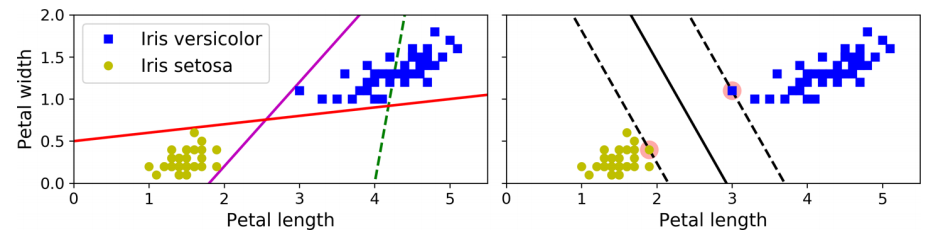
Reviewing the diagram above, you can think of an SVM classifier as fitting the widest possible margin(represented by the parallel dashed lines) between the classes. Margin is the distance between two planes and our goal is to find the widest possible or maximum margin. Intuitively, achieving a wider margin yields lesser generalisation error. The algorithm finds the best possible margin by gaining ‘support’ from data points found along the edges of the margin. Those data points are called support vectors, hence the name, Support Vector Machine. Suppose you delete some points after training and a support vector is affected, the position of the hyperplane would change. This means that the hyperplane drawn is dependent on the position of the support vector. How then is this margin achieved? In logistic regression, we take the output of the linear function and squash the value within the range of [0,1] using the sigmoid function. In SVM, we take the output of the linear function and if that output is greater than 1, we identify it with one class and if the output is -1, we identify is with another class. Since the threshold values are changed to 1 and -1 in SVM, we obtain this reinforcement range of values [-1,1] which acts as the margin.
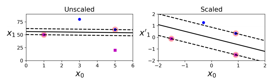
SVMs are sensitive to the feature scales, as you can see above. In the left plot, the vertical scale is much larger than the horizontal scale, so the widest possible margin is close to horizontal. After feature scaling (e.g., using Scikit-Learn’s StandardScaler), the decision boundary in the right plot looks much better. If we strictly impose that all instances must be off the margin and on the right side, this is called hard margin classification. There are two main issues with hard margin classification. First, it only works if the data is linearly separable. Second, it is sensitive to outliers. To avoid these issues, use a more flexible model. The objective is to find a good balance between keeping the margin as large as possible and limiting the margin violations (i.e., instances that end up in the middle of the margin or even on the wrong side). This is called soft margin classification. When creating an SVM model using Scikit-Learn, we can specify a number of hyperparameters. C is one of those hyperparameters. You can practice with this on your own, maybe with a larger dataset. However, note that a model with lots of margin violations will probably not generalize better. If your SVM model is overfitting, you can try regularizing it by reducing C.
from sklearn.svm import SVC

svm_clf = SVC(kernel='linear', random_state=0)

svm_clf.fit(X_train, y_train)
SVC(C=1.0, break_ties=False, cache_size=200, class_weight=None, coef0=0.0,
    decision_function_shape='ovr', degree=3, gamma='scale', kernel='linear',
    max_iter=-1, probability=False, random_state=0, shrinking=True, tol=0.001,
    verbose=False)
svm_pred = svm_clf.predict(X_test)
print( classification_report(y_test, svm_pred) )

print( accuracy_score(y_test, svm_pred))
              precision    recall  f1-score   support

           0       1.00      1.00      1.00        11
           1       1.00      1.00      1.00        13
           2       1.00      1.00      1.00         6

    accuracy                           1.00        30
   macro avg       1.00      1.00      1.00        30
weighted avg       1.00      1.00      1.00        30

1.0
svm_matrix = metrics.confusion_matrix(y_test, svm_pred)
svm_matrix
array([[11,  0,  0],
       [ 0, 13,  0],
       [ 0,  0,  6]], dtype=int64)
4.3 Decision Trees
Like SVMs, Decision Trees are versatile Machine Learning algorithms that can perform both classification and regression tasks, and even multioutput tasks. They are powerful algorithms, capable of fitting complex datasets. In general, a decision tree asks a “Yes or No” question and then makes classification based on the answer. To understand Decision Trees, let’s build one and take a look at how it is trained from a tree graph.
from sklearn.tree import DecisionTreeClassifier

tree_clf = DecisionTreeClassifier(random_state=0)
tree_clf.fit(X_train, y_train)
DecisionTreeClassifier(ccp_alpha=0.0, class_weight=None, criterion='gini',
                       max_depth=None, max_features=None, max_leaf_nodes=None,
                       min_impurity_decrease=0.0, min_impurity_split=None,
                       min_samples_leaf=1, min_samples_split=2,
                       min_weight_fraction_leaf=0.0, presort='deprecated',
                       random_state=0, splitter='best')
#You can visualize the trained Decision Tree by first using the export_graphviz() method to output a graph definition file
#called iris_tree.dot:

feature_names = list(train)
target_names =  iris.Species.unique()

from sklearn.tree import export_graphviz
import pydotplus
from IPython.display import Image

# Export as dot file

dot_data = export_graphviz(tree_clf, out_file=None,
                                feature_names=feature_names,
                                class_names=target_names)
# Draw graph
graph = pydotplus.graph_from_dot_data(dot_data)


# Show graph
Image(graph.create_png())
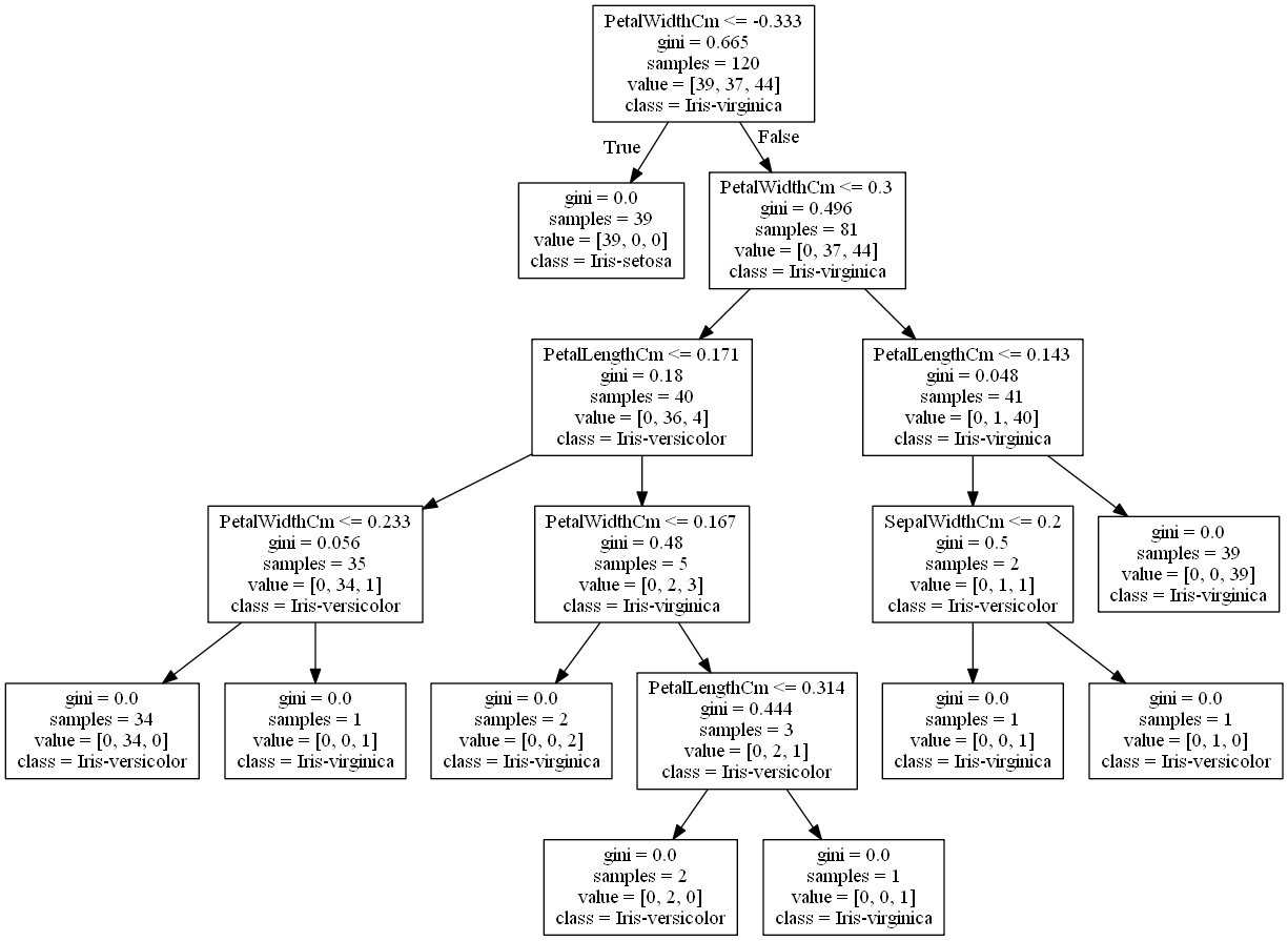
Suppose you find an iris flower and you want to classify it. You start at the root node (depth 0, at the top): this node asks whether the flower’s petal width is smaller than -0.333cm (Remember that we have scaled the dataset, hence negative values). If it is, then you move down to the root’s left child node (depth 1, left). In this case, it is a leaf node (that means it does not have any child nodes), so it does not ask any questions: its simply looks at the predicted class for that node, and the Decision Tree predicts that your flower is an Iris-setosa. Now suppose you find another flower, and this time the petal width is greater than -0.333cm. You must move down to the root’s right child node(depth 1, right), which is not a leaf node, so the node asks another question: is the petal width smaller than 0.3cm? If it is, then your flower is most likely an Iris versicolor (depth 2, left). If not, it is likely an Iris virginica (depth 2, right). To further determine a class for this flower, it goes on to ask about its petal length and so on and so forth. It’s really that simple. A node’s samples attribute counts how many training instances it applies to. For example, 81 training instances have a petal width greater than -0.333cm (depth 1, right), and of those 81, 40 have a petal width smaller than 0.3cm (depth 2, left).
A node’s value attribute tells you how many training instances of each class this node applies to: for example, the node in depth 1 applies to 0 Iris setosa, 37 Iris versicolor, and 44 Iris virginica.
Finally, a node’s gini attribute measures its impurity: a node is “pure” (gini=0) if all training instances it applies to belong to the same class. For example, since the depth-1 left node applies only to Iris setosa training instances, it is pure and its gini score is 0.
The equation below shows how the training algorithm calculates the gini score Gi of the ith node. The depth-2 left node has a gini score equal to 1 – (0/40)2 – (36/40)2 – (4/40)2 = 0.18.
NOTE
Scikit-Learn uses the CART algorithm, which produces only binary trees: non-leaf nodes always have two children (i.e., questions only have yes/no answers).The algorithm works by first splitting the training set into two subsets using a single feature k and a threshold tk (e.g., “petal width ≤ 0.333cm”). How does it choose k and tk? It searches for the pair (k, tk) that produces the purest subsets (weighted by their size). Once the CART algorithm has successfully split the training set in two, it splits the subsets using the same logic, then the sub-subsets, and so on, recursively. It stops “recursing” once it reaches the maximum depth (defined by the max_depth hyperparameter), or if it cannot find a split that will reduce impurity.
As you can see, the CART algorithm is a greedy algorithm: it greedily searches for an optimum split at the top level, then repeats the process at each subsequent level. It does not check whether or not the split will lead to the lowest possible impurity several levels down. A greedy algorithm often produces a solution that’s reasonably good but not guaranteed to be optimal. To avoid overfitting the training data, you need to restrict the Decision Tree’s freedom during training. As you know by now, this is called regularization. The regularization hyperparameters depend on the algorithm used, but generally you can at least restrict the maximum depth of the Decision Tree. In Scikit-Learn, this is controlled by the max_depth hyperparameter (the default value is None, which means unlimited). Reducing max_depth will regularize the model and thus reduce the risk of overfitting. The DecisionTreeClassifier class has a few other parameters that similarly restrict the shape of the Decision Tree: min_samples_split (the minimum number of samples a node must have before it can be split), min_samples_leaf (the minimum number of samples a leaf node must have), min_weight_fraction_leaf (same as min_samples_leaf but expressed as a fraction of the total number of weighted instances), max_leaf_nodes (the maximum number of leaf nodes), and max_features (the maximum number of features that are evaluated for splitting at each node). Increasing min_* hyperparameters or reducing max_* hyperparameters will regularize the model.
tree_pred = tree_clf.predict(X_test)
print( classification_report(y_test, tree_pred) )

print( accuracy_score(y_test, tree_pred))
              precision    recall  f1-score   support

           0       1.00      1.00      1.00        11
           1       1.00      1.00      1.00        13
           2       1.00      1.00      1.00         6

    accuracy                           1.00        30
   macro avg       1.00      1.00      1.00        30
weighted avg       1.00      1.00      1.00        30

1.0
4.4. Ensemble Learning.
Have you watched a television game show called Who wants to be a Millionaire? If no, it goes like this. Basically, you are asked a series of questions where every correct answer gives you some amount of money till you become a millionaire. However, you are given three life lines to help you get to the final stage. One is phone a fried, take a 50:50 chance and ask the audience. In ask the audience, you will find that most players often select answers given by majority of the audience. This is called the wisdom of the crowd which demonstrates how ensemble learning works. Similarly, if you aggregate the predictions of a group of predictors (such as classifiers or regressors), you will often get better predictions than with the best individual predictor. A group of predictors is called an ensemble; thus, this technique is called Ensemble Learning, and an Ensemble Learning algorithm is called an Ensemble method.
4.4.1. Voting Classifiers
Let us assume that you have trained some classifiers as above, each one achieving about 80% accuracy. You have a Logistic Regression classifier, an SVM classifier, a Decision Tree classifier and even a K-Nearest Neighbors classifier.
A very simple way to create an even better classifier is to aggregate the predictions of each classifier and predict the class that gets the most votes. This majority-vote classifier is called a hard voting classifier. Make sure that all classifiers are perfectly independent, making uncorrelated errors, which is clearly not the case because they are trained on the same data. They are likely to make the same types of errors, so there will be many majority votes for the wrong class, reducing the ensemble’s accuracy. TIP Ensemble methods work best when the predictors are as independent from one another as possible. One way to get diverse classifiers is to train them using very different algorithms. This increases the chance that they will make very different types of errors, improving the ensemble’s accuracy.
from sklearn.ensemble import VotingClassifier
from sklearn.neighbors import KNeighborsClassifier

knn_clf = KNeighborsClassifier()
voting_clf = VotingClassifier(
 estimators=[('lr', log_clf), ('dt', tree_clf), ('svc', svm_clf), ('knn', knn_clf)],
 voting='hard')
voting_clf.fit(X_train, y_train)
VotingClassifier(estimators=[('lr',
                              LogisticRegression(C=1.0, class_weight=None,
                                                 dual=False, fit_intercept=True,
                                                 intercept_scaling=1,
                                                 l1_ratio=None, max_iter=500,
                                                 multi_class='multinomial',
                                                 n_jobs=None, penalty='none',
                                                 random_state=0, solver='lbfgs',
                                                 tol=0.0001, verbose=0,
                                                 warm_start=False)),
                             ('dt',
                              DecisionTreeClassifier(ccp_alpha=0.0,
                                                     class_weight=None,
                                                     criterion='...
                                  decision_function_shape='ovr', degree=3,
                                  gamma='scale', kernel='linear', max_iter=-1,
                                  probability=False, random_state=0,
                                  shrinking=True, tol=0.001, verbose=False)),
                             ('knn',
                              KNeighborsClassifier(algorithm='auto',
                                                   leaf_size=30,
                                                   metric='minkowski',
                                                   metric_params=None,
                                                   n_jobs=None, n_neighbors=5,
                                                   p=2, weights='uniform'))],
                 flatten_transform=True, n_jobs=None, voting='hard',
                 weights=None)
#Let’s look at each classifier’s accuracy on the test set:

for clf in (log_clf, tree_clf, svm_clf, knn_clf, voting_clf):
    clf.fit(X_train, y_train)
    y_pred = clf.predict(X_test)
    print(clf.__class__.__name__, accuracy_score(y_test, y_pred))
LogisticRegression 1.0
DecisionTreeClassifier 1.0
SVC 1.0
KNeighborsClassifier 0.9666666666666667
VotingClassifier 1.0
There you go… We can see that the voting classifier produced a perfect classifier by wisdom of the crowd.
4.5.2. Bagging & Pasting.
Another approach of ensemble learning is to train a classifier using random subsets of the dataset. When sampling is performed with replacement, this method is called bagging, short for bootstrap aggregating. When sampling is performed without replacement, it is called pasting. In other words, both bagging and pasting allow training instances to be sampled several times across multiple predictors, but only bagging allows training instances to be sampled several times for the same predictor.
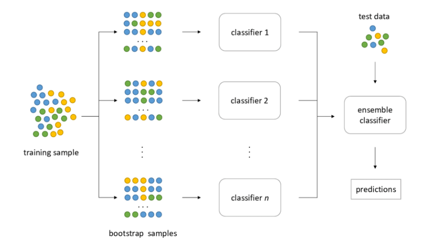
Image Source: hudsonthames.org
Bootstraping creates the foundation of Bagging technique. Bootstrap is a sampling technique in which we select “n” observations out of a population of “n” observations. But the selection is entirely random, i.e., each observation can be chosen from the original population so that each observation is equally likely to be selected in each iteration of the bootstrapping process. After the bootstrapped samples are formed, separate models are trained with the bootstrapped samples. In real experiments, the bootstrapped samples are drawn from the training set, and the sub-models are tested using the testing set. The final output prediction is combined across the projections of all the sub-models.
Once all predictors are trained, the ensemble can make a prediction for a new instance by simply aggregating the predictions of all predictors. The aggregation function is typically the statistical mode (i.e., the most frequent prediction, just like a hard voting classifier) for classification, or the average for regression. Each individual predictor has a higher bias than if it were trained on the original training set, but aggregation reduces both bias and variance. Generally, the net result is that the ensemble has a similar bias but a lower variance than a single predictor trained on the original training set.
Bagging and Pasting in Scikit-Learn
Scikit-Learn offers a simple API for both bagging and pasting with the BaggingClassifier class (or BaggingRegressor for regression). The following code trains an ensemble of 500 Decision Tree classifiers:5 each is trained on 100 training instances randomly sampled from the training set with replacement (this is an example of bagging, but if you want to use pasting instead, just set bootstrap=False). The n_jobs parameter tells ScikitLearn the number of CPU cores to use for training and predictions (–1 tells Scikit-Learn to use all available cores).
from sklearn.ensemble import BaggingClassifier

bag_clf = BaggingClassifier(
 DecisionTreeClassifier(), n_estimators=500, max_samples=100, bootstrap=True, n_jobs=-1, random_state=0)
bag_clf.fit(X_train, y_train)
BaggingClassifier(base_estimator=DecisionTreeClassifier(ccp_alpha=0.0,
                                                        class_weight=None,
                                                        criterion='gini',
                                                        max_depth=None,
                                                        max_features=None,
                                                        max_leaf_nodes=None,
                                                        min_impurity_decrease=0.0,
                                                        min_impurity_split=None,
                                                        min_samples_leaf=1,
                                                        min_samples_split=2,
                                                        min_weight_fraction_leaf=0.0,
                                                        presort='deprecated',
                                                        random_state=None,
                                                        splitter='best'),
                  bootstrap=True, bootstrap_features=False, max_features=1.0,
                  max_samples=100, n_estimators=500, n_jobs=-1, oob_score=False,
                  random_state=0, verbose=0, warm_start=False)
bag_pred = bag_clf.predict(X_test)

print( classification_report(y_test, bag_pred) )

print( accuracy_score(y_test, bag_pred))
              precision    recall  f1-score   support

           0       1.00      1.00      1.00        11
           1       1.00      1.00      1.00        13
           2       1.00      1.00      1.00         6

    accuracy                           1.00        30
   macro avg       1.00      1.00      1.00        30
weighted avg       1.00      1.00      1.00        30

1.0
NOTE The BaggingClassifier automatically performs soft voting instead of hard voting if the base classifier can estimate class probabilities (i.e., if it has a predict_proba() method), which is the case with Decision Tree classifiers.
4.4.3. Random Forests
As an example of an Ensemble method, you can train a group of Decision Tree classifiers, each on a different random subset of the training set. To make predictions, you obtain the predictions of all the individual trees, then predict the class that gets the most votes. Such an ensemble of Decision Trees is called a Random Forest, and despite its simplicity, this is one of the most powerful Machine Learning algorithms available today.
As we have discussed, a Random Forest is an ensemble of Decision Trees, generally trained via the bagging method (or sometimes pasting), typically with max_samples set to the size of the training set. Instead of building a BaggingClassifier and passing it a DecisionTreeClassifier, you can instead use the RandomForestClassifier class, which is more convenient and optimized for Decision Trees (similarly, there is a RandomForestRegressor class for regression tasks). The following code uses all available CPU cores to train a Random Forest classifier with 500 trees (each limited to maximum 16 nodes).
from sklearn.ensemble import RandomForestClassifier
rf_clf = RandomForestClassifier(n_estimators=500, max_leaf_nodes=16, n_jobs=-1)
rf_clf.fit(X_train, y_train)
RandomForestClassifier(bootstrap=True, ccp_alpha=0.0, class_weight=None,
                       criterion='gini', max_depth=None, max_features='auto',
                       max_leaf_nodes=16, max_samples=None,
                       min_impurity_decrease=0.0, min_impurity_split=None,
                       min_samples_leaf=1, min_samples_split=2,
                       min_weight_fraction_leaf=0.0, n_estimators=500,
                       n_jobs=-1, oob_score=False, random_state=None, verbose=0,
                       warm_start=False)
rf_pred = rf_clf.predict(X_test)

print( classification_report(y_test, rf_pred) )

print( accuracy_score(y_test, rf_pred))
              precision    recall  f1-score   support

           0       1.00      1.00      1.00        11
           1       1.00      1.00      1.00        13
           2       1.00      1.00      1.00         6

    accuracy                           1.00        30
   macro avg       1.00      1.00      1.00        30
weighted avg       1.00      1.00      1.00        30

1.0
With a few exceptions, a RandomForestClassifier has all the hyperparameters of a DecisionTreeClassifier (to control how trees are grown), plus all the hyperparameters of a BaggingClassifier to control the ensemble itself. The Random Forest algorithm introduces extra randomness when growing trees; instead of searching for the very best feature when splitting a node as in Decision Tree, it searches for the best feature among a random subset of features. The algorithm results in greater tree diversity, which (again) trades a increased bias for a lower variance, generally yielding an overall better model.
Feature Importance: Yet another great quality of Random Forests is that they make it easy to measure the relative importance of each feature. Scikit-Learn measures a feature’s importance by looking at how much the tree nodes that uses that feature reduce impurity on average (across all trees in the forest). More precisely, it is a weighted average, where each node’s weight is equal to the number of training samples that are associated with it. Scikit-Learn computes this score automatically for each feature after training, then it scales the results so that the sum of all importances is equal to 1. You can access the result using the feature_importances_ variable. For example, the following code trains a RandomForestClassifier on the iris dataset (introduced in Chapter 4) and outputs each feature’s importance. It seems that the most important features are the petal width (44%) and length (43%), while sepal length and width are rather unimportant in comparison.
for name, score in zip(iris[feature_names],
rf_clf.feature_importances_):
    print(name,  score)
SepalLengthCm 0.0975141010857387
SepalWidthCm 0.026917795568990485
PetalLengthCm 0.44788488463059534
PetalWidthCm 0.42768321871467546
4.4.4. Boosting
Boosting (originally called hypothesis boosting) refers to any Ensemble method that can combine several weak learners into a strong learner. The general idea of most boosting methods is to train predictors sequentially, each trying to correct its predecessor. There are many boosting methods available, but by far the most popular are AdaBoost (short for Adaptive Boosting), Gradient Boosting and Extreme Gradient Boosting (Xgb). We will deal with Xgb at a later post. Let’s start with AdaBoost.
4.4.4.a. AdaBoost
One way for a new predictor to correct its predecessor is to pay a bit more attention to the training instances that the predecessor underfitted. This results in new predictors focusing more and more on the hard cases. This is the technique used by AdaBoost. For example, when training an AdaBoost classifier, the algorithm first trains a base classifier (such as a Decision Tree) and uses it to make predictions on the training set. The algorithm then increases the relative weight of misclassified training instances. Then it trains a second classifier, using the updated weights, and again makes predictions on the training set, updates the instance weights, and so on. The algorithm stops when the desired number of predictors is reached, or when a perfect predictor is found. To make predictions, AdaBoost simply computes the predictions of all the predictors and weighs them using the predictor weights αj. The predicted class is the one that receives the majority of weighted votes. Instead of a Decision Tree, AdaBoost uses a Decision Stump which is a decision tree with max_depth = 1, i.e., Tree of single decision node and two leaf nodes. The n_estimators parameters in AdaBoost sets the number of Decision Stumps.
Scikit-Learn uses a multiclass version of AdaBoost called SAMME (which stands for Stagewise Additive Modeling using a Multiclass Exponential loss function). When there are just two classes, SAMME is equivalent to AdaBoost. If the predictors can estimate class probabilities (i.e., if they have a predict_proba() method), Scikit-Learn can use a variant of SAMME called SAMME.R (the R stands for “Real”), which relies on class probabilities rather than predictions and generally performs better. The following code trains an AdaBoost classifier based on 200 Decision Stumps using Scikit-Learn’s AdaBoostClassifier class (as you might expect, there is also an AdaBoostRegressor class).
TIP If your AdaBoost ensemble is overfitting the training set, you can try to reduce the number of estimators or more strongly regularizing the base estimator.
from sklearn.ensemble import AdaBoostClassifier
ada_clf = AdaBoostClassifier(
 DecisionTreeClassifier(max_depth=1), n_estimators=500,
 algorithm="SAMME", learning_rate=0.1)
ada_clf.fit(X_train, y_train)
AdaBoostClassifier(algorithm='SAMME',
                   base_estimator=DecisionTreeClassifier(ccp_alpha=0.0,
                                                         class_weight=None,
                                                         criterion='gini',
                                                         max_depth=1,
                                                         max_features=None,
                                                         max_leaf_nodes=None,
                                                         min_impurity_decrease=0.0,
                                                         min_impurity_split=None,
                                                         min_samples_leaf=1,
                                                         min_samples_split=2,
                                                         min_weight_fraction_leaf=0.0,
                                                         presort='deprecated',
                                                         random_state=None,
                                                         splitter='best'),
                   learning_rate=0.1, n_estimators=500, random_state=None)
ada_pred = ada_clf.predict(X_test)

print( classification_report(y_test, ada_pred))

print( accuracy_score(y_test, ada_pred))
              precision    recall  f1-score   support

           0       1.00      1.00      1.00        11
           1       1.00      1.00      1.00        13
           2       1.00      1.00      1.00         6

    accuracy                           1.00        30
   macro avg       1.00      1.00      1.00        30
weighted avg       1.00      1.00      1.00        30

1.0
4.5.4.b. Gradient Boosting
Another very popular boosting algorithm is Gradient Boosting. Just like AdaBoost, Gradient Boosting works by sequentially adding predictors to an ensemble, each one correcting its predecessor. However, instead of tweaking the instance weights at every iteration like AdaBoost does, this method tries to fit the new predictor to the residual errors made by the previous predictor. Put simply, Fit a model to the given Training set. Calculate the Residual Errors which become the new training instances. A new model is trained on these and so on. An addition of all the models is selected for making predictions.
from sklearn.ensemble import GradientBoostingClassifier

gb_clf = GradientBoostingClassifier(max_depth=2, n_estimators=3, learning_rate=1.0, random_state=42)
gb_clf.fit(X_train, y_train)
GradientBoostingClassifier(ccp_alpha=0.0, criterion='friedman_mse', init=None,
                           learning_rate=1.0, loss='deviance', max_depth=2,
                           max_features=None, max_leaf_nodes=None,
                           min_impurity_decrease=0.0, min_impurity_split=None,
                           min_samples_leaf=1, min_samples_split=2,
                           min_weight_fraction_leaf=0.0, n_estimators=3,
                           n_iter_no_change=None, presort='deprecated',
                           random_state=42, subsample=1.0, tol=0.0001,
                           validation_fraction=0.1, verbose=0,
                           warm_start=False)
gb_pred = gb_clf.predict(X_test)

print( classification_report(y_test, gb_pred))

print( accuracy_score(y_test, gb_pred))
              precision    recall  f1-score   support

           0       1.00      1.00      1.00        11
           1       1.00      1.00      1.00        13
           2       1.00      1.00      1.00         6

    accuracy                           1.00        30
   macro avg       1.00      1.00      1.00        30
weighted avg       1.00      1.00      1.00        30

1.0
5. Conclusion
Whewww… finally… I want to believe that at this stage, you now have a strong grasp of popular machine learning models and you can explain them to none data science colleagues at the office. Till next time, bye for now.
Leave a comment